fit <- fit_fastblm(
  y      = y_sif,        # n observations
  A      = A,            # n x p basis integral matrix
  Q      = Q_sar,        # p x p prior precision
  phi    = phi_hat,      # signal-to-noise: sigma2_b / sigma2_e
  solver = "cholesky"    # "cholesky" | "woodbury" | "pcg"
)

fit$posterior_mean   # p-vector: E[x | y]
fit$sigma2e # estimated noise varianceArea-to-Area Spatial Prediction
fastblm and spatintegrate
Russell Goebel
Predicting new areal averages from areal observations
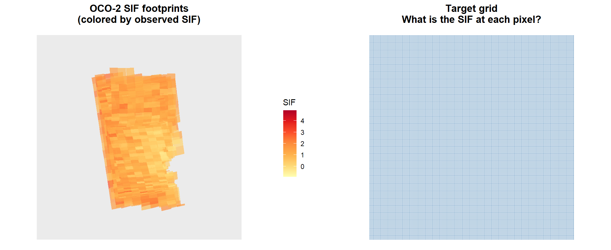
The observations are area averages of the field.
Spatial prediction as a linear model
Whether from a kriging or Gaussian process perspective, spatial prediction can be framed as a Bayesian linear model:
\[y = A x + \varepsilon, \qquad x \sim \mathcal{N}(0,\, \phi\, Q^{-1}), \qquad \varepsilon \sim \mathcal{N}(0,\, \sigma^2_e I)\]
- \(A\) — matrix of basis function integrals: \(A_{ik} = \frac{1}{|D_i|}\int_{D_i}\phi_k(s)\,ds\)
- \(x\) — basis coefficients (coincide with cell values for a raster basis)
- \(Q\) — prior precision on \(x\); any positive-definite matrix
- \(\phi = \sigma^2_b/\sigma^2_e\) — signal-to-noise ratio
The posterior mean \(\hat{x} = \mathbb{E}[x\mid y]\) is the optimal linear predictor. See Kriging is Bayesian linear regression.
Basis function models are especially suited to areal data — they reduce \(O(n^2)\) double integrals over observation polygons to \(O(nK)\) single integrals.
The Heaton et al. (2019) competition
Heaton et al. (2019) compared 12 leading methods on 105,000 satellite surface temperature observations. See my writeup of these methods.
9 of 12 methods fit the \(y = Ax + \varepsilon\) framework:
| Category | Methods |
|---|---|
| Low-rank \(C\) | FRK, Pred. Process, Partitioning, Metakriging |
| Sparse \(C^{-1}\) | SPDE/INLA, LatticeKrig, MRA, NNGP |
| Diagonal via Fourier | Periodic Embedding |
Two performers: SPDE/INLA (the lowest RMSE) and LatticeKrig — both use SAR-like priors on basis coefficients.
Why SAR priors win:
- Sparse \(Q\) via local differential operator
- Matérn covariance emerges from \(( \kappa^2 - \Delta)x = \mathcal{W}\)
- Encodes smoothness without dense precision
This is exactly the prior used in this demo. We also show how to match a Fourier basis to this for grid-free inference.
The Model
\[y = A x + \varepsilon, \qquad x \sim \mathcal{N}(0,\, \phi\, Q^{-1}), \qquad \varepsilon \sim \mathcal{N}(0,\, \sigma^2_e I)\]
- \(y\) — observed SIF values (one per footprint)
- \(A\) — matrix of basis function integrals: \(A_{ik} = \frac{1}{|D_i|}\int_{D_i} \phi_k(s)\,ds\). With a raster basis, \(\phi_k\) is the indicator of pixel \(k\), so \(A_{ik}\) is the overlap fraction.
- \(x\) — basis coefficients. With a raster basis these coincide with grid-cell field values.
- \(\varepsilon\) — i.i.d. Gaussian noise, variance \(\sigma^2_e\)
- \(Q\) — prior precision on \(x\); any positive-definite matrix
- \(\phi = \sigma^2_b / \sigma^2_e\) — signal-to-noise ratio; \(\sigma^2_b\) is the marginal field variance
The posterior mean \(\hat{x} = \mathbb{E}[x \mid y]\) is the optimal linear predictor — equivalent to area-to-area kriging.
Two Packages
fastblm
Fits \(y = Ax + \varepsilon\) for any \(A\) and \(Q\).
- \(A\) is the observation matrix (\(n \times p\))
- \(Q\) is the prior precision on \(x\) (\(p \times p\))
- No special structure assumed
Features:
- CV tuning of \(\phi\) and hyperparameters \(\theta\)
- Cholesky, Woodbury, PCG solvers
- Exact and stochastic posterior SEs
- \(Q\) can be a matrix or operator
spatintegrate
Constructs \(A\) from polygon observations.
\[A_{ik} = \frac{1}{|D_i|}\int_{D_i} \phi_k(s)\, ds\]
Three integration methods:
- Raster overlap — exact polygon intersection
- Fourier — closed-form cosine integrals
- QMC — quasi-random point average
fastblm: Core Function
Returns a fastblm_fit object used by tune_cv and posterior_se.
fastblm: Function Philosophy
Where possible, fastblm accepts operator functions instead of explicit matrices — avoiding materialisation of \(Q^{-1}\).
# Diagonal Q: pass inverse as a function instead of a matrix
fit <- fit_fastblm(...,
  Q     = Diagonal(x = q_diag),
  Q_inv = function(v) v / q_diag   # never forms Q^{-1} explicitly
)

# PCG: Q only needs to be applied as a matrix-vector product
fit <- fit_fastblm(...,
  solver  = "pcg",
  apply_Q = function(v) Q %*% v
)- PCG never stores \(Q^{-1}\) — enables millions of parameters
- Woodbury uses
Q_invto avoid \(p \times p\) solves when \(p \gg n\)
fastblm: Tuning \(\phi\)
# To also tune rho, Q_fun can depend on theta:
Q_fun_rho <- function(theta) {
  rho <- theta[1]
  W   <- make_row_normalised_W(grid)   # row-normalised adjacency
  Q   <- crossprod(Diagonal(p) - rho * W)
  list(Q = Q)
}

# Tune both phi and rho jointly
tuned <- tune_cv(
  y          = y_sif,
  A          = A,
  Q_fun      = Q_fun_rho,
  theta_init = c(rho = 0.99),   # starting value for rho
  k          = 5L,
  verbose    = TRUE
)
tuned$phi     # CV-optimal phi
tuned$theta   # CV-optimal rho
tune_cv optimises \(\phi\) analytically on each fold; \(\theta\) via optim().
fastblm: Three Solvers
\(n\) = observations, \(p\) = basis functions (pixels or modes)
| Solver | When to use | Cost |
|---|---|---|
"cholesky" |
\(p\) small–medium, sparse \(Q\) | \(O(p^{1.5})\) |
"woodbury" |
\(p \gg n\), diagonal \(Q\) | \(O(n^2 p)\) |
"pcg" |
\(p\) very large, \(Q\) cheap to apply | \(O(n_{\text{iter}} \cdot p)\) |
Rule of thumb for this demo:
- Raster SAR (\(p = 28{,}900\) pixels, sparse \(Q\)) →
"cholesky" - Fourier (\(K = 10{,}000\) modes \(\gg n = 6{,}850\) obs, diagonal \(Q\)) →
"woodbury" - Massive raster (millions of cells) →
"pcg"
fastblm: Posterior Standard Errors
Three paths matching the solver:
- Cholesky — exact, reuses cached triangular factor
- Woodbury — exact, reuses cached \(n \times n\) factor. Cost independent of \(p\) — SEs over 28k cells cost the same as 100 cells
- PCG — approximate via Lanczos/Hutchinson. Builds a low-rank approximation to the posterior covariance via Lanczos iteration, then estimates diagonal stochastically. Accuracy controlled by
n_probes.
spatintegrate: Goal
\[A_{ik} = \frac{1}{|D_i|} \int_{D_i} \phi_k(s)\, ds\]
# Raster basis: phi_k = indicator of pixel k -> overlap fractions
A_raster <- compute_overlap_fractions(soundings, grid)

# Fourier basis: phi_k = cos(kx*pi*x) * cos(ky*pi*y) -> exact integrals
A_fourier <- fourier_integrate_basis(soundings, freq_grid)

# General: phi_k evaluated at quasi-random points inside each polygon
A_qmc <- qmc_integrate_basis(soundings, basis, n_points = 5000)spatintegrate: Three Integration Types
Raster overlap
Exact polygon intersection via sf. No approximation.
Best for: SAR/INLA-style raster models.
Fourier / sinusoidal
Closed-form integral of \(\cos(k\pi x)\) over triangulated polygon.
Best for: stationary covariances, large \(K\), irregular prediction geometry.
QMC average
Quasi-random point average of \(\phi_k\) inside polygon.
Best for: non-standard bases, rapid prototyping.
Worked Example: Data
We use projected coordinates for accurate intersection math.
Worked Example: Observation Matrix
Row sums of \(A\) equal 1 — each footprint is fully partitioned across grid cells.
Worked Example: Response
No noise added — raw SIF_757nm observations directly.
Worked Example: SAR Prior
spdep::nb2listw gives a row-normalised weight matrix directly.
rho_fixed <- 0.99

# Row-normalised rook adjacency W
nb  <- spdep::poly2nb(target_proj, queen = FALSE)
lw  <- spdep::nb2listw(nb, style = "W")   # row-normalised
W   <- as(spdep::listw2mat(lw), "sparseMatrix")

# Q = (I - rho*W)'(I - rho*W)
Q_sar <- Matrix::forceSymmetric(
  Matrix::crossprod(Matrix::Diagonal(p) - rho_fixed * W)
)
Q_sar <- Matrix::drop0(Q_sar)
Worked Example: Tune \(\phi\)
Worked Example: Fit SAR Model
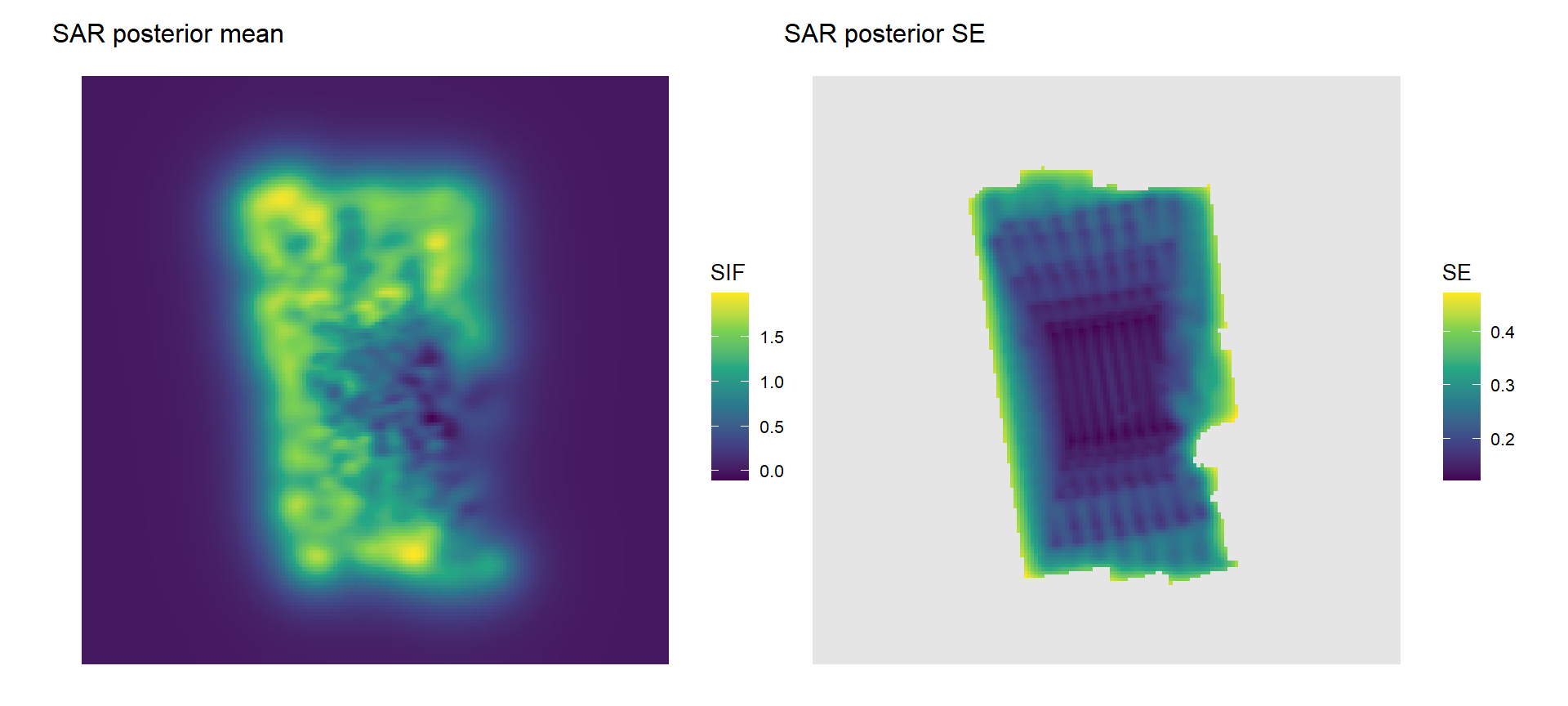
pred_sar is the posterior mean field — one value per grid cell.
Worked Example: Posterior SEs
# Select covered cells via a sparse row-selector matrix
covered_idx <- which(as.numeric(Matrix::colSums(A)) > 0)
A_covered   <- Matrix::sparseMatrix(
  i = seq_along(covered_idx), j = covered_idx,
  x = rep(1, length(covered_idx)),
  dims = c(length(covered_idx), p)
)
se_covered      <- fastblm::posterior_se(fit_sar, A_new = A_covered)
se_sar          <- rep(NA_real_, p)
se_sar[covered_idx] <- se_covered
Worked Example: SAR Results
Switching to a Fourier Basis
Why switch from raster SAR?
- Raster: \(p = 28{,}900\) parameters at this resolution — grows quadratically finer
- Fourier: \(K \ll p\) modes represent the smooth part of the field
- Fourier basis diagonalises all stationary covariances — \(Q\) becomes diagonal
- Predictions at arbitrary locations, not tied to a fixed grid
Key insight: the SAR prior and Matérn covariance both penalise high-frequency modes — they are spectrally equivalent. We can match one to the other exactly.
In this demo: \(K = 10{,}000\) Fourier modes instead of \(p = 28{,}900\) pixels.
Fourier Basis: Prior Matching
\[\kappa^2 = \frac{2d(1-\rho)}{\rho h^2}, \qquad \phi_f = \phi_{\text{SAR}} \cdot \sigma^2_{\text{Matérn}}\]
# Domain: Lx = Ly = 56100m (square), delta = 330m cell size
# J = cells per side; h_norm = normalised cell size on [0,1]^2
L      <- max(Lx, Ly)        # square embedding side (metres)
J      <- round(L / delta)   # cells per side = 170
h_norm <- 1 / J              # normalised cell size = 1/170

# Match SAR prior shape to Matern:
# kappa2 controls spatial range; matern_variance scales amplitude
params      <- get_matern_parameters_from_SAR(rho_fixed,
                 sar_precision = 1, h = h_norm)
KAPPA2_NORM <- params$kappa2
phi_f       <- phi_hat * params$matern_variance

# Spatial range: distance at which correlation ~ 0.1
# In [0,1]^2 units then converted back to metres
sprintf("Spatial range: %.0f m  (kappa2_norm = %.1f)",
        sqrt(8 / (KAPPA2_NORM / L^2)), KAPPA2_NORM)
[1] "Spatial range: 4644 m (kappa2_norm = 1167.7)"Fourier Basis: Frequency Grid
# Square domain bbox in physical CRS coordinates
bbox_sq <- c(target_bbox[1], target_bbox[2],
             target_bbox[1] + L, target_bbox[2] + L)

# Enumerate all (J+1)^2 modes, sort by decreasing prior variance
# (= increasing kappa2_norm + pi^2*(kx^2+ky^2))
kx_all <- rep(0:J, each = J+1L)   # x-frequency index (0 = constant)
ky_all <- rep(0:J, times = J+1L)  # y-frequency index
ord    <- order(KAPPA2_NORM + pi^2 * (kx_all^2 + ky_all^2))

K  <- 10000L   # keep top K modes by prior variance
kx <- kx_all[ord[seq_len(K)]]
ky <- ky_all[ord[seq_len(K)]]

freq_grid <- list(
  omega_mat  = cbind(omega_x = kx*pi/L, omega_y = ky*pi/L),
  norm_const = ifelse(kx==0L,1,sqrt(2)) * ifelse(ky==0L,1,sqrt(2)),
  indices    = cbind(j1=kx+1L, j2=ky+1L),
  J1=max(kx)+1L, J2=max(ky)+1L,
  domain_bbox=bbox_sq, norm="unit_square"
)
Fourier Basis: Integrate and Fit
Fourier Basis: Predictions
# Integrate basis over target grid, multiply immediately
# (avoids storing the full 28900 x 10000 prediction matrix)
future::plan(future::multisession(workers = 4L))
pred_fourier <- as.numeric(
  spatintegrate::fourier_integrate_basis(
    target_proj, freq_grid, parallel = TRUE
  ) %*% fit_f$posterior_mean
)
future::plan(future::sequential())

covered <- lengths(sf::st_intersects(target_proj, soundings_proj)) > 0
r2 <- 1 - sum((pred_fourier[covered] - pred_sar[covered])^2) /
          sum((pred_sar[covered] - mean(pred_sar[covered]))^2)
sprintf("R2(Fourier vs SAR, covered cells): %.4f", r2)
[1] "R2(Fourier vs SAR, covered cells): 0.9997"Same Results, Fewer Parameters
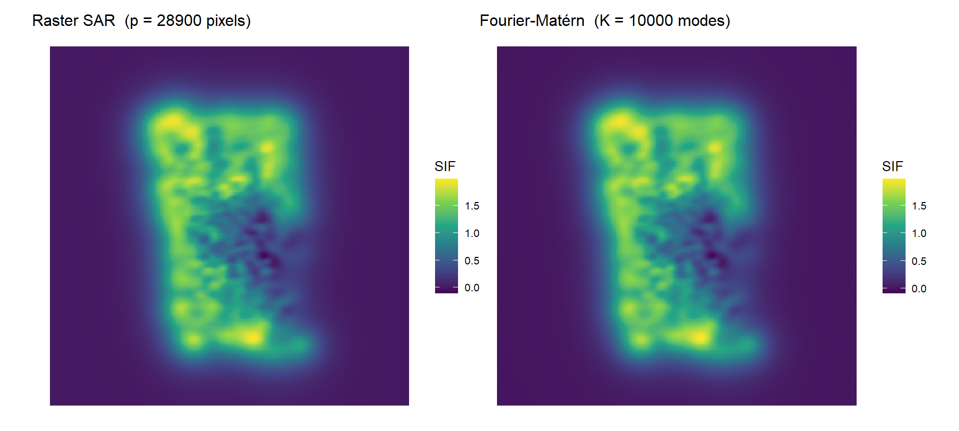
\(K = 10{,}000\) Fourier modes reproduces the \(p = 28{,}900\) pixel SAR prediction.
Conclusion
spatintegratecomputes \(A\) exactly — raster overlaps, Fourier integrals, or QMCfastblmfits \(y = Ax + \varepsilon\) for any \(A\) and \(Q\), with solvers scaling to millions of parameters- Fixed-effect covariates can be included by augmenting \(A\) with a covariate block: \(A = [A_{\text{spatial}} \mid X]\)
- SAR and Matérn priors are spectrally equivalent — switch bases without refitting \(\phi\)
- Fourier basis enables resolution-independent inference and prediction at arbitrary locations