To set the scene: imagine being part of the spatial statistics community, interested in spatial prediction, in 2018.
Optimal prediction methods for the past two decades have centered around Gaussian processes. Methods of optimal prediction have become synonymous with “kriging”, a phrase borrowed from the 1960’s mining community after Danie Krige. These models use a covariance model, and if there are \(n\) observations require an \(O(n^3)\) inversion to fit, let alone to estimate parameters.
That computational complexity is a problem. The spatial statistics community is deeply invested in reducing the \(O(n^3)\), and so decades of research have been done on the topic.
So what is the way to sort through what kinds of methods there are and how well they perform?
In the paper “A Case Study Competition Among Methods for Analyzing Large Spatial Data”, authors of their own methods fit their own procedures on a large-scale dataset — 150,000 simulated observations and then a 105,000 real observation dataset of satellite surface temperatures.
These authors include some heavy-hitters in the spatial statistics community. We’re talking authors of major software packages used for spatial prediction today:
The purpose of this post is to survey each method and try to make clearer the connections between them. In doing so I will link every method to a Bayesian linear model where possible:
Methods that reduce the rank of \(C\)
Fixed-Rank Kriging
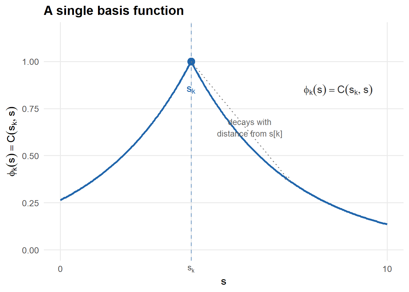
Introduced in 2008 by Cressie & Johannesson, Fixed Rank Kriging begins with a simple observation: any sufficiently smooth spatial field \(v(s)\) can be approximated by a finite basis expansion:
\[v(s) \approx \sum_{k=1}^r \alpha_k \phi_k(s) = \Phi(s)^T \alpha\]
where \(\{\phi_k(s)\}_{k=1}^r\) are fixed basis functions and \(\alpha\) are coefficients. This approximation is never exact — there is a residual:
\[r(s) = v(s) - \Phi(s)^T \alpha\]
representing the part of the field the basis cannot capture. The key insight of FRK is that by choosing \(r \ll n\), all matrix operations reduce from \(O(n^3)\) to \(O(nr^2 + r^3)\).
The full generating model incorporates the approximation error explicitly:
\[y(s) = \mu(s) + \Phi(s)^T \alpha + r(s) + \varepsilon(s)\]
where \(\alpha \sim \mathcal{N}(0, Q^{-1})\) are the basis coefficients with prior precision \(Q\), \(r(s) \sim \mathcal{N}(0, \sigma^2_\xi v(s))\) is the fine-scale residual with known spatially varying weight \(v(s)\) and estimated variance \(\sigma^2_\xi\), and \(\varepsilon(s) \sim \mathcal{N}(0, \sigma^2_\varepsilon)\) is measurement error. Note that \(r(s)\) and \(\varepsilon(s)\) are conceptually distinct — \(r(s)\) represents approximation error from the basis truncation while \(\varepsilon(s)\) represents genuine measurement error — though in practice the two can be difficult to separate.
As a Bayesian Linear model
Exact when \(A = \Phi\).
Deriving \(Q\)
Since \(\Phi Q^{-1} \Phi'\) has rank at most \(r \ll n\), it generally cannot exactly match the target covariance \(C\) — the system \(\Phi Q^{-1} \Phi' = C\) is overdetermined. Instead one seeks the best rank-\(r\) approximation to \(C\). Cressie & Johannesson estimate \(Q^{-1}\) by minimizing the discrepancy between \(\Phi Q^{-1} \Phi'\) and the empirical covariance — a method of moments approach that makes no assumption about the parametric form of \(C\). They note that other choices are possible, and indeed FRK can be seen as a larger umbrella under which several other methodologies fall by choosing \(\Phi\) and \(Q\) cleverly.
Predictive Processes
I’ll motivate predictive processes using the regression framework again. Recall that the kriging predictor can be written as:
\[\hat{x}(s_0) = C(s_0, \mathbf{s}) C^{-1} y = \sum_k \alpha_k C(s_0, s_k)\]
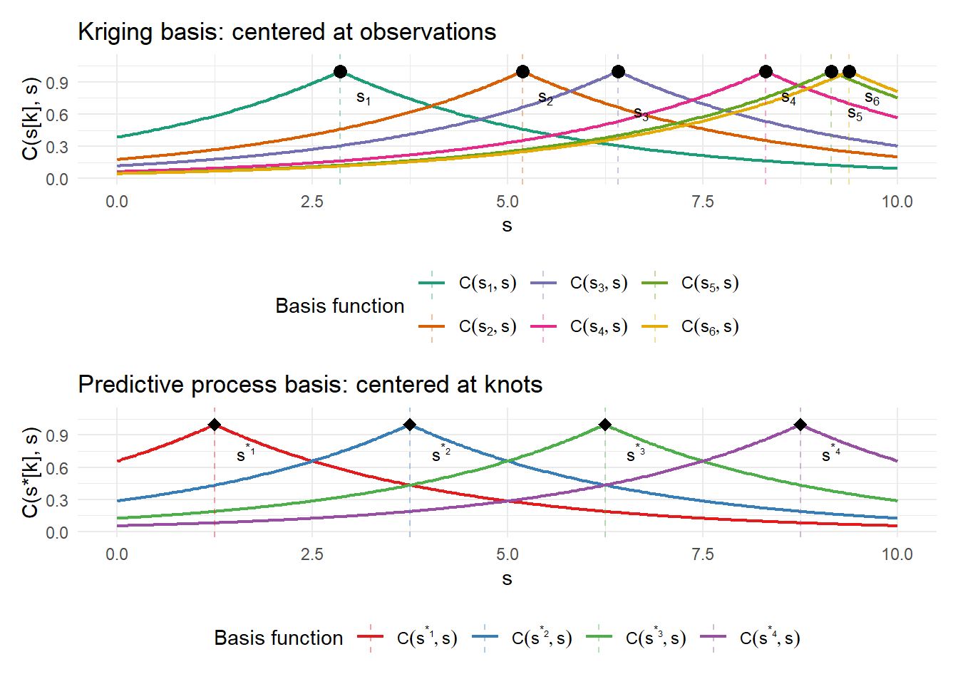
This is equivalent to regressing the observations \(y(s)\) on the basis \(\{C(s_k, s)\}_{k=1}^n\) — one basis function centered at each observation location, with weights \(\alpha = C^{-1}y\) determined by the regression.
This is not accidental. Any covariance function \(C\) defines a Reproducing Kernel Hilbert Space (RKHS) \(\mathcal{H}\), and the representer theorem guarantees that the optimal predictor — the one minimizing squared error subject to fitting the observations — always lives in the span of \(\{C(s_k, \cdot)\}_{k=1}^n\). The observation locations are the natural basis for the solution.
An interesting question arises: “What if instead of centering basis functions at each observation \(s_k\), we choose a different, smaller set of locations \(s_1^*, \ldots, s_m^*\) and use the same basis \(C(s_k^*, s)\)?” In the RKHS context, this amounts to projecting the full kriging predictor onto a lower-dimensional subspace \(\mathcal{H}_m = \text{span}\{C(s_1^*, \cdot), \ldots, C(s_m^*, \cdot)\} \subset \mathcal{H}\) — trading approximation error for computational tractability.
Doing so is exactly Banerjee et al.’s Predictive Processes framework (2008), where this smaller set of locations is called the “knots.” Rather than \(n\) basis functions centered at every observation, we use only \(m \ll n\) basis functions centered at the knots — reducing all matrix operations from \(O(n^3)\) to \(O(nm^2 + m^3)\).
Knot placement is commonly simply done on a regular grid, but there are some more sophisticated approaches.
A correction is sometimes applied as this formulation underestimates the marginal variance.
As a Bayesian Linear Model
The predictive process fits into the \(y = Ax + \varepsilon\) framework with \(A = \Phi\) where \(\Phi_{ik} = C(s_i, s_k^*)\) — cross-covariances between observation locations and knots. The latent field at any location is \(f(s) = \Phi(s)^T \alpha\) where \(\alpha\) are coefficients at the knots.
The implied prior on the field is \(f \sim \mathcal{N}(0, \Phi Q^{-1} \Phi^T)\). Taking \(Q^{-1} = C_{KK}^{-1}\) gives:
\[\Phi Q^{-1} \Phi^T = C_{nK} C_{KK}^{-1} C_{Kn}\]
which is the predictive process covariance — the rank-\(m\) approximation to \(C\) obtained by projecting the full GP prior onto the RKHS subspace spanned by \(\{C(s_k^*, \cdot)\}\). The prior on \(\alpha\) is \(\mathcal{N}(0, C_{KK})\), encoding uncertainty about the knot values before seeing data.
The approximation error is the variance not captured by the projection. The residual process \(\delta(s) = f(s) - \Phi(s)^T \alpha\) has marginal variance
\[C(s,s) - C(s, \mathbf{s}^*)C_{KK}^{-1}C(\mathbf{s}^*, s)\]
at each location — positive everywhere and shrinking toward zero only as the knots become dense. Finley et al. (2009) restore the correct marginal variances by adding this back as a spatially varying diagonal correction, observation by observation, while preserving the rank-\(m\) structure for computation.
Methods that make \(C\) sparse
Spatial Partitioning
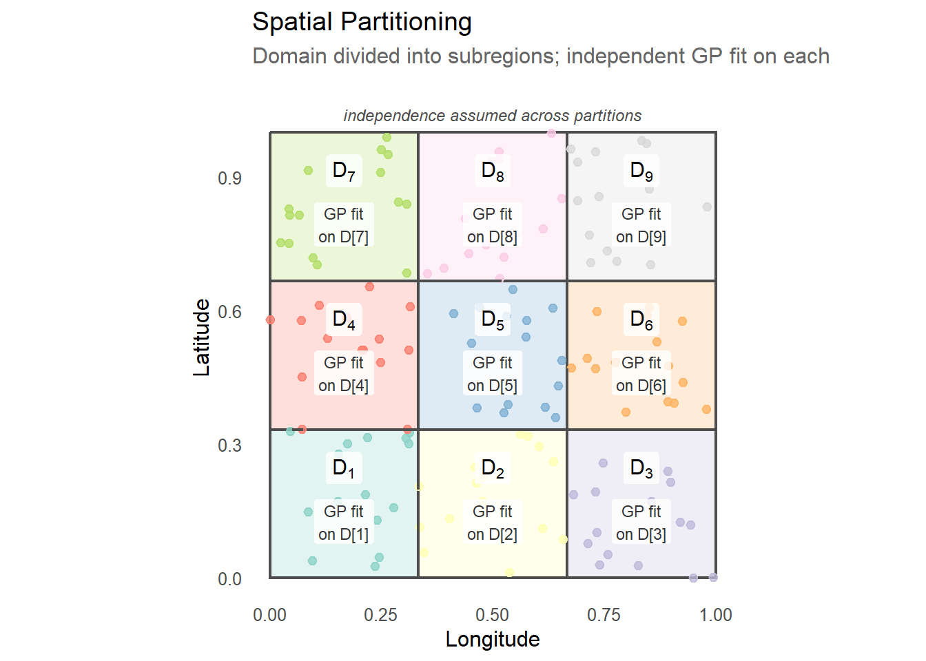
Spatial partitioning takes a different approach to the big-\(n\) problem: rather than approximating the covariance structure globally, it divides the spatial domain into \(D\) non-overlapping subregions and assumes independence across them.
The model within each subregion \(d\) is:
\[y_d = X_d \beta + w_d + \varepsilon_d\]
where \(\beta\) are global regression coefficients shared across all partitions, \(w_d \sim \mathcal{N}(0, \sigma^2 R_d(\theta))\) is a partition-specific spatial process, and \(\varepsilon_d \sim \mathcal{N}(0, \sigma^2_\varepsilon I)\) is measurement error.
The independence assumption across partitions turns the full \(n \times n\) covariance matrix into a block diagonal matrix:
\[C = \begin{pmatrix} C_{11} & & \\ & \ddots & \\ & & C_{DD} \end{pmatrix}\]
This structure reduces the \(O(n^3)\) global inversion to \(D\) independent inversions of \(O((n/D)^3)\) matrices — a quadratic speedup — and the block structure means each partition can be fit in parallel. The likelihood decomposes as a sum over partitions:
\[\log p(y | \theta) = \sum_{d=1}^D \log p(y_d | \theta)\]
which is evaluated independently on each subregion. Importantly, each subregion fit could in principle use any method — exact GP inference, FRK basis functions, NNGP, or any other approximation — making spatial partitioning a meta-strategy rather than a method in its own right. In Heaton’s implementation, exact GP inference is used within each partition.
The shared global parameters \(\beta\) and \(\theta\) couple the partitions together for parameter estimation — the likelihood is block diagonal but the parameter estimates depend on all partitions simultaneously. This is what distinguishes spatial partitioning from metakriging: in metakriging each subset is fit completely independently with its own parameters, while spatial partitioning shares parameters globally across partitions.
Limitations
The partition independence assumption means the model cannot represent spatial correlations that extend across partition boundaries. Predictions near boundaries tend to be discontinuous and predictive variance is underestimated where the true correlation structure spans multiple partitions. The coverage of 0.86 in the Heaton results reflects this — the model is overconfident near boundaries. Unlike metakriging, there is no correction step to recover cross-partition information after the fit.
As a Bayesian Linear Model
Spatial partitioning fits exactly into the \(y = Ax + \varepsilon\) framework, with \(A = I\) and the approximation living entirely in \(C\). The full covariance matrix is replaced by a block diagonal version:
\[C \approx C_{block} = \begin{pmatrix} C_{11} & & \\ & \ddots & \\ & & C_{DD} \end{pmatrix}\]
where \(C_{dd} = \{C(s_i, s_j)\}_{s_i, s_j \in \mathcal{D}_d}\) is the exact covariance matrix within partition \(d\), and all cross-partition covariances are set to zero. The prior on \(x\) is then \(x \sim \mathcal{N}(0, C_{block})\) and the posterior mean is:
\[\hat{x} = C_{block}(C_{block} + \sigma^2_\varepsilon I)^{-1} y\]
which decomposes into \(D\) independent systems — one per partition — each of size \(n/D \times n/D\). This is exact kriging within each partition, with the approximation being the assumption that \(C_{block} \approx C\).
The global parameters \(\beta\) and \(\theta\) enter through \(C_{block}(\theta)\) and the mean \(X\beta\), coupling the partitions for parameter estimation even though the posterior decomposes independently given \(\theta\).
Covariance Tapering
The motivating insight behind covariance tapering is that \(C(s, t)\) is approximately zero when \(s\) and \(t\) are far apart — so why not zero it out explicitly, since including nearly-negligible covariances is computationally expensive?
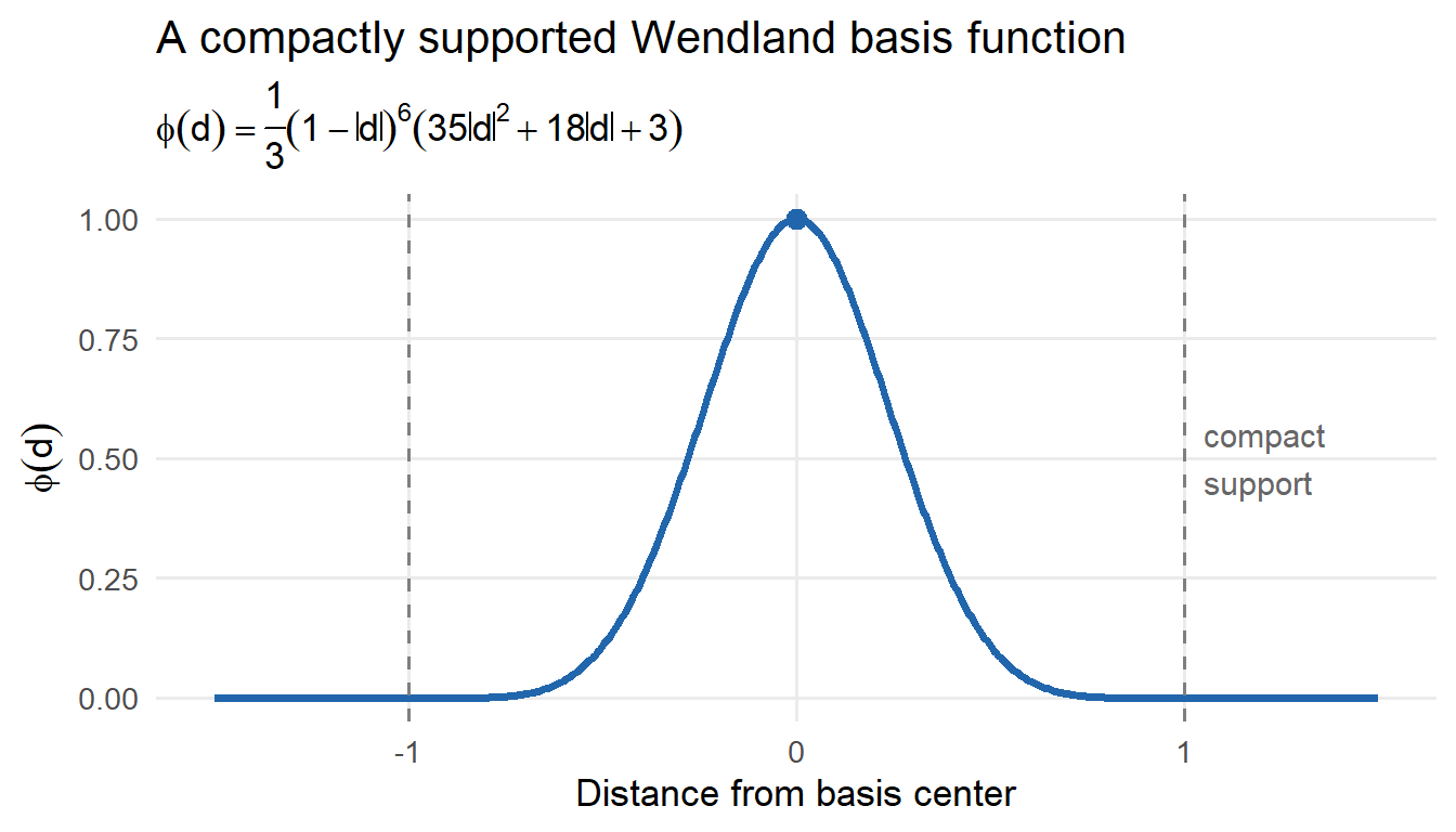
There are a few nuances however. Multiplying \(C(s,t)\) by an arbitrary compactly supported function \(T(s,t)\) does not necessarily result in a valid covariance function — the product may not be positive semi-definite, which would prevent Cholesky decomposition. To guarantee that \(C(s,t) \cdot T(s,t)\) is a valid covariance function, \(T(s,t)\) is itself chosen to be a valid compactly supported covariance function. The Hadamard product of two valid covariance functions is always a valid covariance function — this is the key result that makes tapering principled. Common choices for \(T\) include the Wendland family of compactly supported covariances.
A second nuance concerns parameter estimation. If \(C(\theta)\) is replaced by the tapered version \(C(\theta) \cdot T\), maximizing the resulting likelihood no longer recovers the true parameters \(\theta\) — the estimates correspond to a misspecified model where long-range correlations are absent. To obtain unbiased parameter estimates, the two-taper approach of Kaufman et al. (2008) also tapers the empirical covariance in the likelihood:
\[\ell(\theta) \propto -\log|C(\theta) \cdot T| -
\text{tr}\left[(C(\theta) \cdot T)^{-1} \{(y - \mu)(y-\mu)^T \cdot T\}\right]\]
This gives unbiased estimating equations at the cost of some computational efficiency. The simpler one-taper approach tapers only \(C(\theta)\), which is faster but introduces bias in parameter estimates that can affect predictive performance.
As a Bayesian Linear Model
\(A = I\), with the approximation living entirely in \(C\) — the tapered covariance \(C \cdot T\) replaces the full \(C\). The sparsity of \(C \cdot T\) allows Cholesky factorization in \(O(n \cdot \text{nnz})\) rather than \(O(n^3)\), where \(\text{nnz}\) is the number of nonzero entries per row determined by the taper range.
Methods that make \(C^{-1}\) Sparse
Stochastic Partial Differential Equations (SPDE)
The SPDE approach, introduced by Lindgren, Rue & Lindström (2011), begins from a remarkable theoretical result: a Gaussian random field with Matérn covariance is the solution to a specific stochastic partial differential equation. For a field \(x(s)\) on \(\mathbb{R}^2\):
\[(\kappa^2 - \Delta)^{\alpha/2} x(s) = \mathcal{W}(s)\]
where \(\Delta\) is the Laplacian, \(\kappa > 0\) controls the range, \(\alpha = \nu + 1\) for smoothness \(\nu\), and \(\mathcal{W}(s)\) is Gaussian white noise. The connection to the Matérn family is exact for integer \(\alpha\) and approximate otherwise.
The key insight is that this differential operator is local — it only involves relationships between nearby points. Discretizing it via finite elements therefore produces a sparse precision matrix \(Q\), giving computational tractability without approximating the covariance function itself.
Discretization and the connection to SAR/CAR models
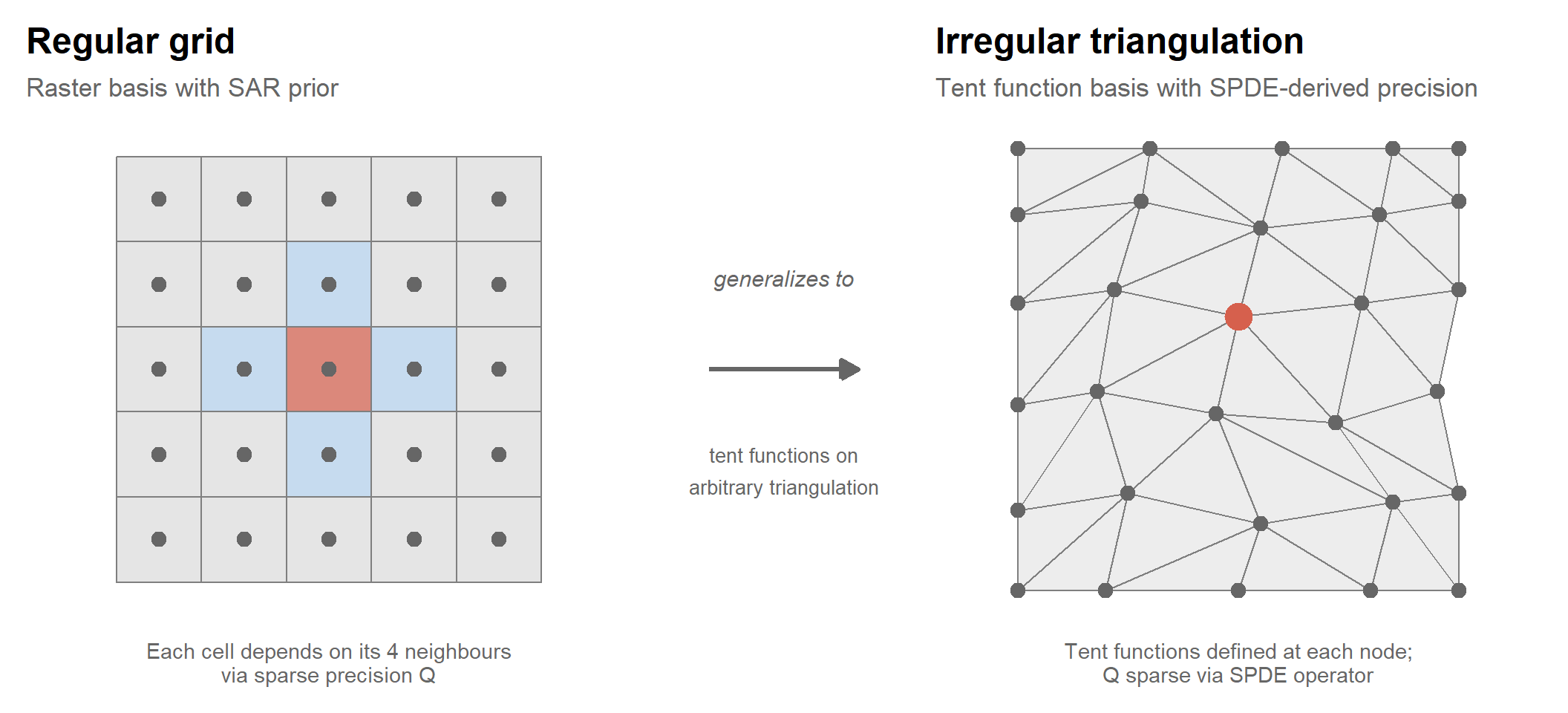
To make this concrete, consider discretizing the SPDE on a regular grid — the simplest case. The Laplacian \(\Delta\) at interior grid point \(s_i\) is approximated by finite differences:
\[\Delta x(s_i) \approx x(s_{i-1,j}) + x(s_{i+1,j}) + x(s_{i,j-1}) + x(s_{i,j+1}) - 4x(s_i)\]
Substituting into the SPDE for \(\alpha = 2\) (\(\nu = 1\)) gives:
\[(\kappa^2 - \Delta) x(s_i) = (\kappa^2 + 4)x(s_i) - \sum_{j \in N(i)} x(s_j) = \mathcal{W}(s_i)\]
In matrix form this is exactly a Simultaneous Autoregressive (SAR) model. Rearranging the finite difference equation:
\[(\kappa^2 + 4)x_{ij} = x_{i-1,j} + x_{i+1,j} + x_{i,j-1} + x_{i,j+1} + \varepsilon_{ij}\]
we can write this as \(x = Wx + \varepsilon\) where \(W\) is the row-normalized adjacency matrix with \(W_{ij} = \frac{1}{\kappa^2 + 4}\) for each neighbour \(j\) of \(i\). In matrix form:
\[Bx = \varepsilon, \quad \varepsilon \sim \mathcal{N}(0, \sigma^2 I)\]
where \(B = I - W = \frac{1}{\kappa^2 + 4}(\kappa^2 I - \Delta_h)\) is a scaled version of the discrete Laplacian \(\Delta_h\). The precision matrix is \(Q = B^T B / \sigma^2\), which is sparse because \(B\) has at most 5 nonzero entries per row — the cell itself and its 4 neighbours. The implied covariance \(Q^{-1}\) is dense, encoding long-range spatial correlations that propagate through the local neighbourhood structure of \(B\).
where \(B_{ii} = \kappa^2 + 4\) and \(B_{ij} = -1\) for neighbors \(j \in N(i)\). The precision matrix is \(Q = B^T B / \sigma^2\) — sparse, with nonzeros only among neighboring grid cells.
This is the \(y = Ax + \varepsilon\) framework with \(A = B^{-1}\) — but more usefully written in precision form. The SAR model is the natural discretization of the SPDE on a regular grid via finite differences — the approximation improves as the grid spacing shrinks to zero. The implied covariance \(Q^{-1}\) approximates the Matérn covariance with smoothness \(\nu = 1\).
For \(\alpha = 1\) (\(\nu = 0\), exponential-like) the operator is \((\kappa^2 - \Delta)^{1/2}\) which requires a fractional power — this is where the non-integer case becomes approximate, as discussed in the context of the Heaton comparison.
A Conditional Autoregressive (CAR) model is the symmetric version, specifying the conditional distributions directly:
\[x(s_i) | x(s_{-i}) \sim \mathcal{N}\left(\sum_{j \in N(i)} w_{ij} x(s_j), \tau^2\right)\]
which gives precision matrix \(Q_{ij} = -w_{ij}/\tau^2\) for \(i \neq j\) and \(Q_{ii} = 1/\tau^2\). CAR models are the GMRF version of the same idea — specifying the field through local conditional distributions rather than a global autoregression.
The triangulation mesh
On irregular observation locations, the SPDE is discretized using finite elements on a triangulation mesh. Piecewise linear (tent) basis functions \(\phi_k(s)\) are defined at each mesh node, and the field is approximated as:
\[x(s) \approx \sum_k \alpha_k \phi_k(s)\]
The finite element discretization of the SPDE operator produces a sparse precision matrix \(Q\) for the coefficients \(\alpha\), with nonzeros only between nodes connected by a mesh edge. Prediction at any location \(s_0\) is then:
\[\hat{x}(s_0) = \sum_k \phi_k(s_0) \hat{\alpha}_k = \Phi(s_0)^T \hat{\alpha}\]
which is exactly the \(Ax + \varepsilon\) framework with \(A_{ik} = \phi_k(s_i)\) — a sparse matrix since each observation falls in exactly one triangle and activates only its three corner nodes.
As a Bayesian Linear Model
\(A = \Phi\) (sparse finite element evaluation matrix), \(x = \alpha\) (field coefficients at mesh nodes), \(x \sim \mathcal{N}(0, Q^{-1})\) where \(Q\) is the sparse SPDE precision. The approximation lives entirely in \(C^{-1} = Q\) — the covariance is never formed explicitly.
LatticeKrig
LatticeKrig can be motivated as a smooth multiresolution extension of the SAR/SPDE viewpoint.
Recall from the SPDE discussion that sparse autoregressive models on a lattice grid naturally induce spatial dependence. On a regular raster, one may write the field as
\[
g(s)
=
\sum_{k=1}^m c_k I_k(s)
\]
where: - \(I_k(s)\) is the indicator function for raster cell \(k\), - and \(c_k\) is the latent value associated with that cell.
A sparse autoregressive prior is then placed on the coefficients:
\[
Bc = \varepsilon
\]
where \(B\) encodes local neighborhood structure on the grid. This induces a sparse precision matrix:
\[
Q = B^T B
\]
exactly as in SAR, CAR, and SPDE models. Although the precision is sparse, the implied covariance \(Q^{-1}\) is globally supported, allowing long-range spatial dependence to emerge through repeated local interactions.
The key insight of the SPDE approach is that these local autoregressive constructions approximate Matérn Gaussian fields under mesh refinement.
From raster cells to smooth basis functions
The problem with the raster representation above is that the basis functions are discontinuous and not smooth. The resulting field is piecewise constant and can exhibit visible grid artifacts. The tent functions in Lindgren would be continuous, but not smooth.
LatticeKrig replaces the indicator basis functions with smooth compactly supported basis functions:
\[
g(s)
=
\sum_{k=1}^m c_k \phi_k(s)
\]
where \(\phi_k(s)\) are Wendland basis functions centered on a lattice grid.
Because the Wendland functions are compactly supported: - each basis function affects only a local neighborhood, - the basis evaluation matrix remains sparse, - and the resulting field becomes smooth rather than blocky.
The coefficients \(c_k\) still follow a sparse autoregressive prior, so the model preserves the computational advantages of sparse precision matrices while producing a continuous spatial surface.
This viewpoint makes LatticeKrig resemble a smooth finite-element version of the SPDE/SAR framework: - sparse local dependence is imposed on coefficients, - compactly supported basis functions interpolate those coefficients into a continuous field, - and long-range covariance emerges implicitly through the sparse precision structure.
Why multiple resolutions?
A single sparse lattice is already capable of producing globally correlated spatial fields. In principle, one resolution level is sufficient to induce long-range dependence.
The motivation for multiple resolutions is therefore not to create long-range covariance, but to represent spatial variation across many scales more efficiently.
A single fine-resolution lattice can represent both broad smooth variation and local detail, but doing so is computationally inefficient:
- large-scale structure requires many local coefficients,
- low-frequency variation is poorly represented using only highly localized basis functions,
- and computations become unnecessarily expensive.
LatticeKrig instead introduces multiple resolutions:
\[
g(s)
=
\sum_{\ell=1}^L g_\ell(s)
=
\sum_{\ell=1}^L
\sum_{k=1}^{m_\ell}
c_{k,\ell}\phi_{k,\ell}(s)
\]
where: - coarse resolutions capture broad smooth structure, - finer resolutions capture increasingly localized detail, - and each level has its own sparse autoregressive structure.
Unlike MRA methods, these levels are not recursive residual corrections. Instead, the latent processes at different resolutions are modeled as independent additive components:
\[
\text{Cov}(g_\ell(s), g_{\ell'}(t)) = 0,
\quad \ell \neq \ell'
\]
so the covariance becomes
\[
\text{Cov}(g(s), g(t))
=
\sum_{\ell=1}^L
\text{Cov}(g_\ell(s), g_\ell(t)).
\]
This multiresolution structure is reminiscent of wavelet decompositions: - coarse levels efficiently represent low-frequency variation, - fine levels efficiently represent high-frequency local structure, - and the combination yields flexible Matérn-like spatial behavior.
As a Bayesian Linear Model
LatticeKrig fits naturally into the Bayesian linear model framework:
\[
y = A x + \varepsilon
\]
with: - \(A = \Phi\), the sparse basis evaluation matrix, - \(x = c\), the stacked basis coefficients across resolutions, - and \(\varepsilon \sim \mathcal N(0, \sigma^2 I)\).
The approximation lives primarily in: - the sparse autoregressive precision matrices placed on the coefficients, - and the multiresolution compactly supported basis representation.
Multiresolution Approximations (MRA)
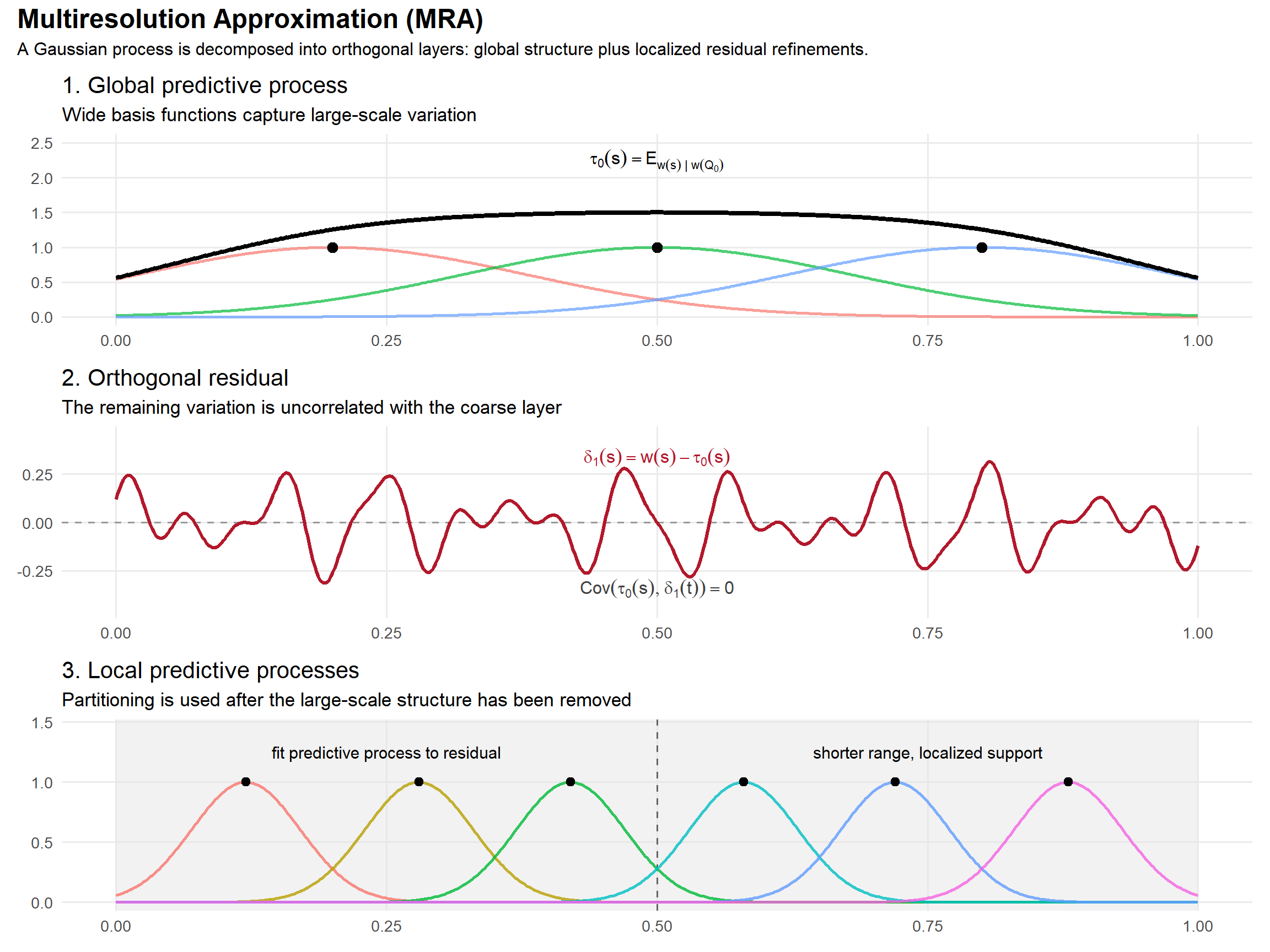
The multiresolution approach used in the Heaton competition is deeply connected to predictive processes.
Recall that a predictive process approximates a Gaussian process using a small number of knot locations:
\[
\tau_0(s)
=
E[w(s)\mid w(\mathcal Q_0)]
\]
where \(\mathcal Q_0\) is a set of coarse knots. This captures the large-scale structure of the process while reducing computation from \(O(n^3)\) to \(O(nm^2 + m^3)\).
However, this approximation is not exact. There is a residual:
\[
\delta_1(s)
=
w(s)-\tau_0(s)
\]
representing the variation not captured by the coarse knots.
The key insight behind multiresolution approximations is that this residual is orthogonal to the predictive process itself:
\[
\text{Cov}(\tau_0(s), \delta_1(t)) = 0
\]
because conditional expectation is an orthogonal projection in \(L^2\). This means we can model the residual separately without creating a fully coupled dense covariance structure.
Importantly, the residual process has a shorter correlation range than the original process. The coarse predictive process already explains the long-range spatial dependence, so the remaining variation is increasingly local.
This suggests a recursive strategy:
- Fit a coarse predictive process.
- Compute the residual.
- Approximate the residual using a second predictive process with more localized knots.
- Repeat.
The resulting representation resembles a wavelet or multigrid decomposition for Gaussian processes: coarse global structure is modeled first, while increasingly localized basis functions refine the remaining variation.
A multiresolution expansion therefore takes the form
\[
w(s)
=
\sum_{r=0}^{R}
\sum_{k=1}^{m_r}
b_{r,k}(s)\eta_{r,k}
\]
where: - \(r\) indexes the resolution level, - coarse resolutions have broad spatial support, - fine resolutions have increasingly local support, - and \(\eta_{r,k}\) are Gaussian coefficients.
The multiresolution aspect enters through domain partitioning. At coarse resolutions, basis functions may span the entire spatial domain. At finer resolutions, the domain is recursively partitioned into subregions, and basis functions are localized within those subregions.
This localization induces sparsity: - coarse basis functions are globally supported but few in number, - fine-scale basis functions are numerous but each affects only a small region, - each observation interacts with only a small number of fine-scale basis functions.
As a result, the basis evaluation matrix becomes increasingly sparse at finer resolutions.
Unlike simple spatial partitioning, MRA does not assume independence between distant regions. Long-range dependence is carried through the coarse resolutions, while fine-scale local structure is handled through localized residual corrections.
Computationally, MRA achieves scalability through sparse precision and sparse basis interaction structure rather than by directly sparsifying the covariance itself. The covariance of the implied process remains globally supported even though the computations become local.
As a Bayesian Linear Model
MRA fits naturally into the Bayesian linear model framework:
\[
y = A x + \varepsilon
\]
with: - \(A = \Phi\), the multiresolution basis evaluation matrix, - \(x = \eta\), the stacked basis coefficients across resolutions, - and \(\varepsilon \sim \mathcal N(0, \sigma^2 I)\).
The approximation lies in the structured multiresolution prior placed on the coefficients \(\eta\). Coarse-resolution coefficients induce long-range dependence, while fine-resolution coefficients induce local corrections.
The resulting design matrix has a characteristic hierarchical sparsity pattern: - the coarsest basis functions interact with nearly all observations, - intermediate resolutions interact with subsets of the domain, - and the finest resolutions interact only locally.
This produces sparse matrix operations while still preserving large-scale spatial dependence.
Nearest Neighbor Gaussian Processes (NNGP)
Nearest Neighbor Gaussian Processes begin with a remarkably simple observation: every multivariate density can be written as a product of conditional densities.
Suppose
\[
w =
(w_1,\ldots,w_n)^T.
\]
Then the joint density can always be factorized as
\[
p(w)
=
p(w_1)
\prod_{i=2}^n
p(w_i \mid w_1,\ldots,w_{i-1}).
\]
This identity is exact and does not depend on Gaussianity.
For a Gaussian process, however, the conditional distributions take a particularly convenient form. If
\[
w \sim \mathcal N(0,C),
\]
then each conditional distribution is Gaussian:
\[
w_i \mid w_1,\ldots,w_{i-1}
\sim
\mathcal N(B_i w_{1:i-1}, F_i)
\]
where
\[
B_i
=
C_{i,1:i-1}
C_{1:i-1,1:i-1}^{-1}
\]
and
\[
F_i
=
C_{ii}
-
C_{i,1:i-1}
C_{1:i-1,1:i-1}^{-1}
C_{1:i-1,i}.
\]
Thus the exact Gaussian process can be viewed as a sequence of regressions:
\[
w_i
=
B_i w_{1:i-1}
+
\eta_i,
\qquad
\eta_i \sim \mathcal N(0,F_i),
\]
where each location is regressed on all previous locations.
The problem is computational. As (i) grows, the conditioning sets become larger and larger. Eventually every point depends on nearly every previous point, reproducing the familiar (O(n^3)) computational cost of Gaussian process inference.
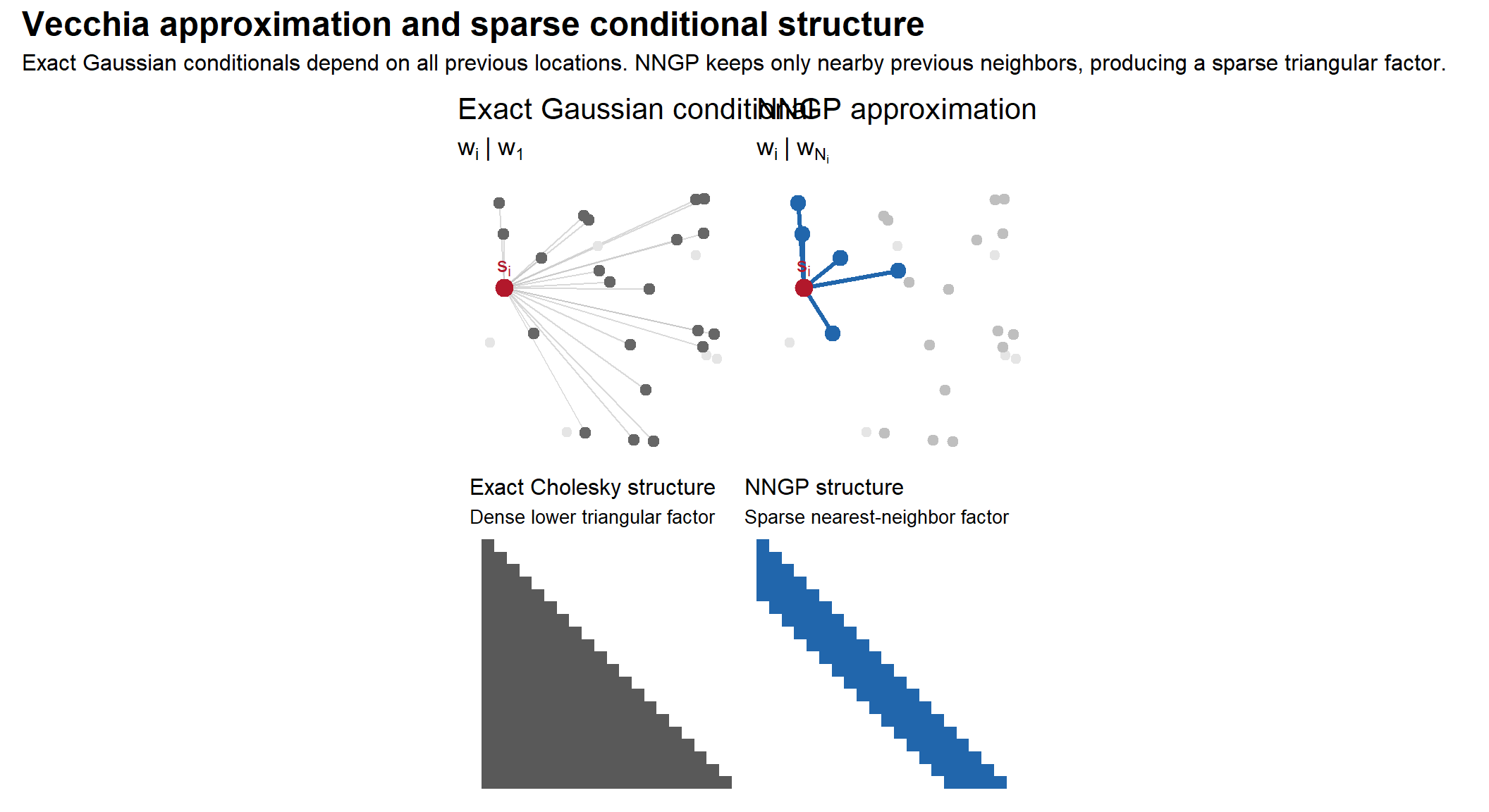
The Vecchia approximation
The key idea of Vecchia (1988) is that most of those conditional dependencies are unnecessary.
Spatially distant observations contribute relatively little once nearby observations are known. Therefore, instead of conditioning on all previous locations, we approximate each conditional using only a small neighbor set:
\[
p(w_i \mid w_1,\ldots,w_{i-1})
\approx
p(w_i \mid w_{N_i}),
\]
where (N_i {1,,i-1}) contains only a small number of nearby previous locations.
This gives the approximate joint density
\[
\tilde p(w)
=
p(w_1)
\prod_{i=2}^n
p(w_i \mid w_{N_i}).
\]
The ordering is essential. Each point may only condition on previous locations, ensuring the resulting dependency graph is a directed acyclic graph (DAG). This guarantees that the approximation still defines a valid joint Gaussian distribution.
The nearest-neighbor Gaussian process applies this approximation directly to Gaussian process models. For each location (s_i), the neighbor set (N_i) typically contains the (m) nearest previous locations in space.
The approximate conditional distribution becomes
\[
w_i \mid w_{N_i}
\sim
\mathcal N(B_i^{(N)} w_{N_i}, F_i^{(N)}),
\]
where
\[
B_i^{(N)}
=
C_{i,N_i}
C_{N_i,N_i}^{-1}
\]
and
\[
F_i^{(N)}
=
C_{ii}
-
C_{i,N_i}
C_{N_i,N_i}^{-1}
C_{N_i,i}.
\]
Equivalently,
\[
w_i
=
B_i^{(N)} w_{N_i}
+
\eta_i,
\qquad
\eta_i \sim \mathcal N(0,F_i^{(N)}).
\]
Sparse Cholesky structure
The important computational consequence is that these regressions are now sparse.
In the exact Gaussian process, each (w_i) depends on nearly all previous locations, so the regression coefficients form a dense lower-triangular system. Under the nearest-neighbor approximation, each location depends on only (m) nearby locations.
Stacking the regression equations yields
\[
Aw = \eta,
\]
where: - (A) is sparse and lower triangular, - each row contains only (m+1) nonzero entries, - and (N(0,F)) with (F) diagonal.
The implied precision matrix is therefore
\[
Q
=
A^T F^{-1} A,
\]
which is sparse.
This is the key conceptual point of NNGP: - the covariance matrix remains dense, - but the conditional dependence structure becomes sparse.
Long-range spatial dependence is still present implicitly. Nearby locations influence one another directly, and information propagates globally through chains of local neighbors.
Relationship to other sparse precision methods
NNGP is philosophically similar to SPDE and GMRF approaches: - all replace dense global dependence with sparse local dependence, - all produce sparse precision matrices, - and all retain globally correlated spatial fields.
The difference is primarily conceptual: - SPDE methods begin from local differential operators, - while NNGP begins from sparse approximations to Gaussian conditional distributions.
Unlike predictive process or fixed-rank methods, NNGP does not reduce the dimension of the latent field. There is still one latent variable per observation location. Scalability instead comes entirely from sparsifying the conditional regression structure.
As a Bayesian Linear Model
NNGP fits naturally into the Bayesian linear model framework:
\[
y = A x + \varepsilon
\]
with: - (x = w), the latent spatial process evaluated at observation locations, - and (w N(0,Q^{-1})) where (Q) is sparse.
The approximation therefore lives entirely in the sparse precision structure induced by the nearest-neighbor conditional factorization.
Periodic Embedding
Every method discussed so far approximates the covariance matrix \(C\) in some way — making it low-rank, sparse, or sparse in its inverse. Periodic embedding takes a fundamentally different route: it does nothing to \(C\) at all. Instead it chooses a basis in which \(C\) is already diagonal, making every matrix operation trivially cheap.
The key observation is that for a stationary process on a regular grid, the covariance matrix is circulant — each row is a cyclic shift of the row above it. Circulant matrices are diagonalized exactly by the discrete Fourier transform:
\[C = \Phi \, \mathrm{diag}(\Lambda) \, \Phi^H\]
where \(\Phi\) is the DFT matrix and \(\Lambda_k = S(\omega_k)\) is the spectral density evaluated at frequency \(\omega_k\). The spectral density of a Matérn-1/2 process, for example, has the closed form \(S(\omega) \propto \sigma^2 \ell / (1 + (2\pi\ell\omega)^2)\), decaying as \(1/\omega^2\) — so the low frequencies carry most of the variance and high frequencies are shrunk heavily toward zero.
In the Bayesian linear model \(y = \Phi x + \varepsilon\), \(x \sim \mathcal{N}(0, \mathrm{diag}(\Lambda))\), the prior on \(x\) is diagonal by construction: different frequency components have independent amplitudes. The likelihood also factors across frequencies when \(y\) is observed on the complete regular grid, because the DFT of white noise is white noise — \(\mathrm{DFT}(\varepsilon)_k\) are independent across \(k\). Independent prior times factored likelihood gives an independent posterior: each \(x_k\) updates from its own frequency component of the data \(\hat{y}_k = \mathrm{DFT}(y)_k\) alone, with posterior mean and variance
\[\mu_k = \frac{\Lambda_k \hat{y}_k}{\Lambda_k + N\sigma^2_\varepsilon}, \qquad \mathrm{Var}[x_k] = \frac{\Lambda_k N \sigma^2_\varepsilon}{\Lambda_k + N\sigma^2_\varepsilon}.\]
This is the complete posterior — \(N\) independent scalar Gaussians rather than one joint \(N\)-dimensional Gaussian. The usual \(O(n^3)\) matrix inversion has been replaced by \(N\) scalar divisions.
Two complications: edge effects and missing data
The circulant structure requires two conditions: stationarity (which we assume anyway) and a complete regular grid. In practice neither holds exactly.
The first issue is edge effects. On a finite domain, the circulant assumption wraps the covariance periodically — the field at the left boundary is treated as correlated with the field at the right boundary. This introduces bias in spectral estimates. The fix is to embed the observation domain into a slightly larger periodic domain, expanding each dimension by a factor \(\tau \geq 1\). Guinness & Fuentes (2017) show that \(\tau\) as small as 1.1 or 1.25 is sufficient — a remarkably small expansion that adds few artificial grid points.
The second issue is missing data. Real gridded datasets, like the satellite surface temperature data in the Heaton competition, have missing values wherever clouds obscure the sensor or land pixels fall inside the ocean domain. On an incomplete grid the DFT of the partial data is no longer separable by frequency — knowing \(\hat{y}_k\) from the observed subset mixes contributions from all frequencies because the incomplete sum destroys the sinusoidal orthogonality.
The Guinness (2019) solution is iterative imputation. At each iteration, missing values are imputed under the current spectral model, the complete grid is formed, the periodogram is updated, and the process repeats. Concretely, the algorithm is:
- Initialize with a flat spectrum.
- Conditionally simulate missing grid values \(y_{miss}\) given \(y_{obs}\) under the current spectral model.
- Compute the periodogram of the complete grid and smooth it to update the spectrum estimate.
- Repeat until convergence.
Each step costs \(O(N \log N)\) via the FFT, and the method never forms or inverts any matrix. In the Heaton competition this was among the fastest methods — 13 minutes total, competitive with methods that assumed known covariance parameters — and achieved the best interval score of all competitors.
As a Bayesian linear model
In the unified \(y = Ax + \varepsilon\) framework, periodic embedding sits in a different cell of the taxonomy than every other method. The matrix \(A = \Phi^H / N\) is the IDFT matrix — dense, but structured. The prior \(x \sim \mathcal{N}(0, \mathrm{diag}(\Lambda))\) is diagonal. The approximation lives not in \(A\), \(C\), or \(C^{-1}\) directly, but in the observation model: the method requires a complete regular grid, so missing values must be imputed to make \(A^H A = (1/N)I\) hold exactly. It is the only method in the Heaton comparison where the computational gain comes entirely from basis choice rather than covariance approximation.
Algorithmic Approaches (no global covariance model)
Local Approximate Gaussian Processes (laGP)
Every method discussed so far builds a global model — some approximation to the full \(n \times n\) covariance structure that is then used to predict everywhere. laGP (Gramacy & Apley 2015) takes the opposite approach: rather than approximating the global model, it abandons it entirely and fits a separate small exact GP for each prediction location.
For a target location \(s_0\), laGP selects a neighborhood \(\mathcal{N}(s_0)\) of \(m \ll n\) nearby observations, fits an exact GP on those \(m\) points, and produces a prediction. The neighborhood is chosen greedily to maximize predictive information — at each step adding the observation that most reduces posterior variance at \(s_0\). With \(m\) fixed (typically \(m \approx 50\)), each prediction costs \(O(m^3)\) regardless of \(n\), and predictions at different locations are embarrassingly parallel.
The approximation is not in the covariance model or the basis — it is in which data you condition on. The local GP uses the exact Matérn covariance, exact inference, and exact uncertainty quantification, but throws away all observations beyond the neighborhood as if they were independent of \(s_0\) given \(\mathcal{N}(s_0)\). This is philosophically similar to NNGP — both exploit the intuition that distant observations carry little information once nearby ones are known — but the implementation is completely different. NNGP constructs a single global sparse precision matrix encoding all the local dependencies at once. laGP constructs nothing globally at all, solving a fresh \(m \times m\) system per prediction location.
As a Bayesian linear model
laGP resists the \(y = Ax + \varepsilon\) framing because there is no global \(x\). Each prediction is its own model. If forced into the framework you could write \(A = I_{(m)}\) restricted to the local neighborhood, but this obscures more than it reveals. It is cleaner to say laGP is the one method in the Heaton comparison that never forms \(C\) at all — not approximately, not sparsely, not in a transformed basis. The global covariance structure is simply never computed.
In the Heaton results laGP was competitive on point prediction but slower than spectral methods due to the per-location cost, and uncertainty quantification was reasonable. Its main advantage is conceptual simplicity and exact local inference; its main disadvantage is that predictions at nearby locations share no computation and the method does not produce a coherent joint predictive distribution over the domain.
Gapfill
Gapfill (Gerber et al. 2018) is included in the Heaton comparison for completeness but sits outside the probabilistic framework of every other method. It is an algorithmic gap-filling procedure designed specifically for satellite raster data: missing pixels are imputed using quantile regression on spatiotemporal neighbors, with the quantile chosen to match the observed marginal distribution of the data. There is no likelihood, no prior, no posterior — just a fast nonparametric interpolation scheme.
It does not fit the \(y = Ax + \varepsilon\) framework and is not a Gaussian process method in any sense. Its inclusion in the Heaton comparison reflects the practical reality that many practitioners filling gaps in satellite data reach for fast algorithmic tools rather than probabilistic models. In the results, Gapfill was very fast but had the largest interval score of all methods — its predictive intervals were wide and poorly calibrated — which is unsurprising given that it was not designed for uncertainty quantification.