Kriging is Bayesian Linear Regression

A unified view of kriging, GP regression, and spatial basis function methods

1 Introduction

1.1 Kriging as Bayesian Linear Regression

In this post, I make the claim that “Kriging–a method so dominant in the field of geostatistics as to be almost synonymous with spatial prediction–is Bayesian linear regression.” This is a bit provocative in that kriging does not require distributional assumptions and is not typically framed in Bayesian terms. But the claim is still precise: for any kriging method producing a prediction \(p\) and prediction error \(s\), there exists a Bayesian linear regression model with a Gaussian prior whose posterior mean is \(p\) and posterior standard deviation is \(s\).

If you don’t find this provocative, another reaction you might have is “this is obvious.” It may be more accurate and familiar to use the terminology “Gaussian process regression” instead of “Bayesian Linear Regression” (as I write this the Wikipedia page for Kriging even reads, “Kriging, or Gaussian Process Regression”). But this raises two questions: first, even introductory Kriging texts often point out that a Gaussian assumption is unnecessary (so how can Kriging be GP regression?), and second, if GP regression is typically described in Bayesian terms, as they are taught in Rasmussen and Williams (2006) , how can it produce the same results as Kriging, which is still typically presented from a frequentist perspective?

If you’re in the former camp, it may be helpful distinguish between two things:

• 1. Kriging as a mathematical object, consisting of spatial predictions and prediction properties uniquely satisfying a notion of optimality from a given statistical formulation,
• 2. Kriging as a modeling philosophy, that is, a collection of procedures that range from parameter fitting to common problem-setup choices.

When I say “Kriging is Bayesian linear regression”, I mean it purely in the first way, though in this post I hope to acknowledge some of the traditions in (ii) and a few trade-offs that might occur. I am not alone in reducing “kriging” to the prediction itself. In Stein (1999), Stein writes, “Best linear unbiased prediction is frequently used in spatial statistics where it is commonly called universal kriging”, and more directly “Best linear unbiased prediction is called kriging in the geostatistical literature”. In N. A. C. Cressie (1993), Cressie writes, “Kriging is synonymous with optimal prediction.” It may be unsurprising to a Bayesian that there is a link with posterior means and variance and a BLUE estimate. Yet, the distinction between i. and ii. also brings another question: kriging procedures historically used distinct fitting procedures, such as those using the variogram; and they also tend to bring discussions of sources of error (“epistemic vs aleatoric error”) which are sometimes directly encoded in the model. So, what differences in modelling traditions are there, and how much do they matter in practice?

The structure of this post is as follows:

• The explicit correspondence — how to construct the underlying matrices to recover simple, ordinary, universal, fixed-rank, and area-to-area kriging as special cases of the same Bayesian linear regression model, including several state-of-the-art methods for scaling to large-\(n\).
• Statistical traditions in kriging and GP regression — the modeling choices that distinguish the two literatures in practice, such as the variogram, parameter estimation, and the nugget effect. Along the way we resolve the two questions raised above: why the Gaussian assumption does not change the prediction, and why frequentist and Bayesian derivations produce identical formulas.
• A history of spatial prediction — kriging and Gaussian process regression as parallel developments across three communities, visualised in an interactive timeline.
• Numerical verification — demonstrating the matrix solves implied by the linear model for simple kriging and the SPDE approach match popular software implementations.

Without further fanfare…

1.2 Explicit correspondence between Kriging and a Bayesian linear model

Consider the Bayesian linear regression model with known covariance matrix

\[y = A\alpha + \varepsilon, \quad \alpha \sim N(0, Q^{-1}), \quad \varepsilon \sim N(0, \Sigma)\]

whose posterior mean and variance are:

\[\hat{\alpha} = (A^T \Sigma^{-1}A + Q)^{-1} A^T\Sigma^{-1}y\]

\[\text{Var}(\alpha \mid y, Q, \Sigma) = (A^T\Sigma^{-1}A + Q)^{-1}\] In the following tabset panels, how to choose A and Q to match various kriging models is given. For these panels I choose a more straightforward way of expressing kriging predictions with a linear model (using identity matrices as designs and augmenting with prediction locations), but there is an equivalent functional version using covariance functions as basis functions which connects to reproducing kernel Hilbert spaces. Several of the methods discussed here are drawn from Heaton et al. (2019), a noteworthy paper in which the authors of each method implemented their own procedure and competed head-to-head on both simulated and real satellite surface temperature data.

Simple kriging

State vector

\[\alpha = (v_\text{obs},\ v(s_0))^\top\]

Observation matrix

\[A = \begin{pmatrix} I & 0 \end{pmatrix}\]

Prior precision

\[Q = Q_{\text{all}}, \qquad Q_{\text{all}} = \begin{pmatrix} \Sigma_{\text{obs}} & k(s_0) \\ k(s_0)^\top & C(s_0, s_0) \end{pmatrix}^{-1}\]

Mean assumption: Known, zero mean.

Computational cost: \(O(n^3)\) — dense matrix inversion.

Prediction at \(s_0\) is \(e_{n+1}^\top\hat{\alpha}\) — reading off the last component of the posterior mean.

\[\hat{v}(s_0) = e_{n+1}^\top(Q + A^\top\Sigma^{-1}A)^{-1} A^\top\Sigma^{-1} y\]

Ordinary kriging

State vector

\[\alpha = (\mu,\ v_\text{obs},\ v(s_0))^\top\]

Observation matrix

\[A = \begin{pmatrix} \mathbf{1} & I & 0 \end{pmatrix}\]

Prior precision

\[Q = \begin{pmatrix} 0 & 0 \\ 0 & Q_{\text{all}} \end{pmatrix}\]

The zero block encodes a flat (improper) prior on \(\mu\); \(Q_{\text{all}}\) is as defined in the Simple Kriging tab.

Mean assumption: Unknown constant mean \(\mu\).

Computational cost: \(O(n^3)\) — dense matrix inversion.

The full prediction adds the estimated mean to the residual field. The prediction vector \(c\) picks out both \(\mu\) and \(v(s_0)\):

\[\hat{u}(s_0) = c^\top(Q + A^\top\Sigma^{-1}A)^{-1} A^\top\Sigma^{-1} y, \qquad c = \begin{pmatrix} 1 \\ 0_n \\ 1 \end{pmatrix}\]

Universal kriging

State vector

\[\alpha = (\beta,\ v_\text{obs},\ v(s_0))^\top\]

Observation matrix

\[A = \begin{pmatrix} F & I & 0 \end{pmatrix}, \qquad F_{ij} = f_j(s_i)\]

Prior precision

\[Q = \begin{pmatrix} 0_p & 0 \\ 0 & Q_{\text{all}} \end{pmatrix}\]

The \(p \times p\) zero block encodes a flat (improper) prior on \(\beta \in \mathbb{R}^p\); \(Q_{\text{all}}\) is as defined in the Simple kriging tab.

Mean assumption: Unknown mean \(\mu(s) = f(s)^\top\beta\).

Computational cost: \(O(n^3)\) — dense matrix inversion.

The full prediction combines the trend \(f(s_0)^\top\hat{\beta}\) with the residual field \(\hat{v}(s_0)\):

\[\hat{u}(s_0) = c^\top(Q + A^\top\Sigma^{-1}A)^{-1} A^\top\Sigma^{-1} y, \qquad c = \begin{pmatrix} f(s_0) \\ 0_n \\ 1 \end{pmatrix}\]

Ordinary kriging is the special case \(f(s) = 1\), \(p = 1\).

Fixed-rank kriging

Contributed by Andrew Zammit-Mangion to the Heaton et al. (2019) case study competition.

Paper: N. Cressie and Johannesson (2008); Zammit-Mangion and Cressie (2021)

Package: FRK

Approximation: Low-rank \(C\) — bisquare basis functions, \(Q\) estimated by method of moments

---

State vector

\[\alpha = (\alpha_1, \ldots, \alpha_r)^\top\]

Observation matrix

\[A = \Phi_{\text{obs}}, \qquad A_{ij} = \phi_j(s_i)\]

where \(\phi_j\) are bisquare basis functions at multiple resolutions, centered on a regular grid.

Prior precision

\[Q \in \mathbb{R}^{r \times r}\]

Estimated by method of moments: \(Q^{-1}\) is chosen so that \(\Phi Q^{-1} \Phi^\top\) best approximates the empirical covariance. No parametric form of \(C\) is assumed.

Mean assumption: Known, zero mean.

Computational cost: \(O(nr^2 + r^3)\) — tractable when \(r \ll n\).

Prediction evaluates the basis at the target location directly:

\[\hat{v}(s_0) = \phi(s_0)^\top(Q + A^\top\Sigma^{-1}A)^{-1} A^\top\Sigma^{-1} y\]

Notes: FRK had the worst RMSE on simulated data (1.31) among GP methods. The bisquare basis lives outside the RKHS of the covariance function, so the method of moments \(Q\) has no principled connection to the true Matérn covariance — unlike Predictive Processes whose basis functions are covariance evaluations and whose \(Q = C_{KK}^{-1}\) is the RKHS inner product.

Predictive Process

Contributed by Andrew Finley to the Heaton et al. (2019) case study competition.

Paper: Banerjee et al. (2008); Finley et al. (2009)

Package: spBayes

Approximation: Low-rank \(C\) — covariance basis functions at knots, RKHS projection

---

State vector

\[\alpha = (v(s_1^*), \ldots, v(s_m^*))^\top\]

Latent field values at the \(m\) knot locations.

Observation matrix

\[A = C_{nK}, \qquad A_{ik} = C(s_i, s_k^*)\]

Cross-covariances between observation locations and knots.

Prior precision

\[Q = C_{KK}^{-1}\]

The prior on \(\alpha\) is \(\mathcal{N}(0, C_{KK})\) — the GP prior restricted to the knots. The implied prior on the field is \(f \sim \mathcal{N}(0, C_{nK} C_{KK}^{-1} C_{Kn})\), the rank-\(m\) projection of the full GP prior onto the RKHS subspace spanned by \(\{C(s_k^*, \cdot)\}\).

Mean assumption: Known, zero mean.

Computational cost: \(O(nm^2 + m^3)\).

Prediction at \(s_0\) uses the cross-covariance row \(C(s_0, \mathbf{s}^*)\):

\[\hat{v}(s_0) = C(s_0, \mathbf{s}^*)\,(Q + A^\top\Sigma^{-1}A)^{-1} A^\top\Sigma^{-1} y\]

Variance correction: The marginal variance deficit at each location is \(C(s_i, s_i) - C(s_i, \mathbf{s}^*)C_{KK}^{-1}C(\mathbf{s}^*, s_i)\). Finley et al. (2009) add this back as a spatially varying diagonal correction, observation by observation, while preserving the rank-\(m\) structure.

Notes: Worst RMSE on both datasets (1.43 simulated, 2.64 satellite). The global knot set is a degenerate Vecchia conditioning set — the same \(m\) knots for every observation — which is why it performs poorly relative to methods with local conditioning.

Spatial Partitioning

Contributed by Matthew Heaton to the Heaton et al. (2019) case study competition.

Paper: Heaton et al. (2019)

Package: —

Approximation: Low-rank \(C\) — block diagonal covariance, independence across partitions

---

State vector

\[\alpha = (v_\text{obs},\ v(s_0))^\top\]

For \(A = I\) methods, including \(v(s_0)\) in the state vector and augmenting \(Q_{\text{all}}\) to include \(s_0\) gives prediction as \(e_{n+1}^\top \hat{\alpha}\) with no separate kriging step required.

Observation matrix

\[A = \begin{pmatrix} I & 0 \end{pmatrix}\]

Prior precision

\[Q = C_{\text{block}}^{-1}, \qquad C_{\text{block}} = \begin{pmatrix} C_{11} & & \\ & \ddots & \\ & & C_{DD} \end{pmatrix}\]

Cross-partition covariances are set to zero. Each \(C_{dd}\) is the exact Matérn covariance within partition \(d\).

Mean assumption: Unknown constant \(\mu\) shared globally across partitions (flat prior).

Computational cost: \(D\) independent \(O((n/D)^3)\) inversions — quadratic speedup.

Notes: Heaton used a \(10 \times 20\) grid of partitions (200 cells, ~746 observations each). Predictions near partition boundaries are discontinuous — cross-partition covariance is zero by assumption. Coverage of 0.86 on simulated data reflects overconfidence near boundaries. Shares global \((\sigma^2, \theta)\) across partitions, unlike Metakriging where each partition has its own parameters.

Covariance Tapering

Contributed by Reinhard Furrer to the Heaton et al. (2019) case study competition.

Paper: Furrer, Genton, and Nychka (2006); Kaufman, Schervish, and Nychka (2008)

Package: spam

Approximation: Sparse \(C\) — Hadamard product with compact Wendland taper

---

State vector

\[\alpha = (v_\text{obs},\ v(s_0))^\top\]

As with all \(A = I\) methods, including \(v(s_0)\) in the state vector and augmenting \(Q_{\text{all}}\) to include \(s_0\) gives prediction directly from the posterior mean — no separate kriging step.

Observation matrix

\[A = \begin{pmatrix} I & 0 \end{pmatrix}\]

Prior precision

\[Q = (C \cdot T)^{-1}\]

where \(C \cdot T\) denotes the Hadamard product of the Matérn covariance with a compactly supported Wendland taper. The Hadamard product of two valid covariances is a valid covariance, guaranteeing positive definiteness.

Mean assumption: Known, zero mean.

Computational cost: \(O(n \cdot \text{nnz})\) sparse Cholesky, where \(\text{nnz}\) is determined by the taper range.

Notes: The one-taper approach (taper only \(C\)) introduces parameter bias. The two-taper approach of Kaufman, Schervish, and Nychka (2008) additionally tapers the empirical covariance, giving unbiased estimating equations at some computational cost. Heaton used the two-taper approach. Coverage was 1.00 on simulated data — the taper inflates predictive variance by discarding long-range information.

SPDE (point-to-point)

Contributed by Finn Lindgren to the Heaton et al. (2019) case study competition.

Paper: Lindgren, Rue, and Lindström (2011)

Package: R-INLA

Approximation: Sparse \(C^{-1}\) — SPDE operator discretised on triangulation mesh

---

State vector

\[\alpha = (\alpha_1, \ldots, \alpha_K)^\top\]

Coefficients at \(K\) mesh nodes.

Observation matrix

\[A = \Phi_{\text{obs}}, \qquad A_{ij} = \phi_j(s_i)\]

Sparse: each observation falls in exactly one triangle and activates only its 3 corner nodes.

Prior precision

\[Q = (\kappa^2 I + \Delta_h)^{2\nu} / c\]

Sparse banded precision from Lindgren, Rue, and Lindström (2011). On a regular grid this recovers the SAR/CAR stencil exactly: \(B_{ii} = \kappa^2 + 4\), \(B_{ij} = -1\) for neighbours, \(Q = B^\top B / \sigma^2\).

Mean assumption: Known, zero mean.

Computational cost: \(O(K^{3/2})\) for sparse Cholesky on the 2D mesh.

Prediction evaluates tent functions at \(s_0\):

\[\hat{v}(s_0) = \phi(s_0)^\top(Q + A^\top\Sigma^{-1}A)^{-1} A^\top\Sigma^{-1} y\]

Notes: Won the satellite dataset (RMSE 1.53) but coverage of 1.00 on simulated data. Root cause: mesh spacing ~6 miles vs data grid ~0.5 miles (10× coarser). With ~100 observations per mesh node, the fine-scale differences that identify the nugget are destroyed. A fine mesh matching data spacing would cost ~96 days. The practical fix is to pre-estimate or fix the nugget before fitting SPDE on dense gridded data.

ATA kriging (general)

Not part of the Heaton et al. (2019) competition — included here as an extension of the SPDE framework explored in this post, showing how the BLM handles areal observations.

Observation model

\[y_i = \frac{1}{|B_i|}\int_{B_i} v(s)\,ds + \varepsilon_i\]

Each observation is an areal average of the field over footprint \(B_i\) — a linear functional of \(v\), not a matrix-vector product. \(A\) cannot be written in closed form without a basis representation of \(v\).

Prior precision

\[Q^{-1}_{ij} = \frac{1}{|B_i||B_j|}\int_{B_i}\int_{B_j} C(s,t)\,ds\,dt\]

Computational cost: \(O(n^2 m^2)\) to form \(Q^{-1}\) where \(m\) is quadrature points per footprint, then \(O(n^3)\) to invert.

\[\hat{L}_0[v] = k_0^\top(K + \Sigma)^{-1} y, \qquad K_{ij} = \frac{1}{|B_i||B_j|}\int_{B_i}\int_{B_j} C(s,t)\,ds\,dt\]

SPDE (area-to-area)

Not part of the Heaton et al. (2019) competition — included here as an extension showing how switching from point to areal observations only changes \(A\), not \(Q\), within the Lindgren, Rue, and Lindström (2011) framework.

Observation matrix

\[A_{ij} = \frac{1}{|B_i|}\int_{B_i} \phi_j(s)\,ds\]

Target row

\[a_{0j} = \frac{1}{|B_0|}\int_{B_0} \phi_j(s)\,ds \quad \text{(block target)} \qquad \text{or} \qquad a_{0j} = \phi_j(s_0) \quad \text{(point target)}\]

Prior precision

\[Q = (\kappa^2 I + \Delta_h)^{2\nu} / c\]

Same sparse banded \(Q\) as the point case — only \(A\) changes for areal observations.

Computational cost: \(O(nKm)\) single integrals to build \(A\), then sparse solve. Replaces the \(O(n^2 m^2)\) double integrals of exact ATA kriging.

\[\hat{L}_0[v] = a_0^\top(Q + A^\top\Sigma^{-1}A)^{-1} A^\top\Sigma^{-1} y\]

LatticeKrig

Contributed by Douglas Nychka to the Heaton et al. (2019) case study competition.

Paper: Nychka et al. (2015)

Package: LatticeKrig

Approximation: Sparse \(C^{-1}\) — Wendland basis on regular lattice, SAR prior

---

State vector

\[\alpha = (c_1, \ldots, c_K)^\top\]

Stacked Wendland coefficients across \(L\) resolution levels, \(K = \sum_\ell m_\ell\) total.

Observation matrix

\[A = \Phi, \qquad A_{ik} = \phi_k(s_i)\]

Sparse Wendland \(C^4\) basis: \(\phi(d) = \frac{1}{3}(1-d)^6(35d^2 + 18d + 3)\) for \(d \leq 1\), zero otherwise.

Prior precision

\[Q = \mathrm{bdiag}(Q_1, \ldots, Q_L), \qquad Q_\ell = B_\ell^\top B_\ell\]

SAR prior on each level: \(B_{jj} = 4 + \kappa^2\), \(B_{jk} = -1\) for lattice neighbours. Levels are independent. A single resolution level has fixed smoothness; the multiresolution sum approximates arbitrary Matérn spectral decay (Theorem 4.1, Nychka et al. 2015).

Mean assumption: Known, zero mean.

Computational cost: Sparse \(A\) and \(Q\) give \(O(nK)\) formation and \(O(K)\) sparse solve. Heaton used NC=40, nlevel=4, \(K \approx 136{,}000\).

Prediction evaluates the Wendland basis at \(s_0\):

\[\hat{v}(s_0) = \phi(s_0)^\top(Q + A^\top\Sigma^{-1}A)^{-1} A^\top\Sigma^{-1} y\]

Uncertainty: Heaton’s implementation uses \(M = 100\) conditional simulations; posterior variance estimated as variance across draws plus nugget \(\sigma^2_{MLE}\) added separately. Avoids forming \(A \Sigma_\alpha A^\top\) explicitly.

Notes: RMSE 0.87 simulated, 1.68 satellite, coverage 0.97 — well calibrated.

MRA

Contributed by Matthias Katzfuss & Dorit Hammerling to the Heaton et al. (2019) case study competition.

Paper: Katzfuss (2017); Katzfuss and Guinness (2021)

Package: GPvecchia

Approximation: Sparse \(C^{-1}\) — recursive predictive processes, block-sparse precision

---

State vector

\[\alpha = (\eta_{0,1}, \ldots, \eta_{0,m_0},\ \eta_{1,1}, \ldots, \eta_{R,m_R})^\top\]

Stacked coefficients across \(R+1\) levels. The coarsest level (\(r=0\)) is a global predictive process covering the whole domain; each finer level models the orthogonal residual locally within recursively partitioned cells.

Observation matrix

\[A = \Phi, \qquad A_{ik} = C(s_i, s_k^{(r)})\]

Hierarchically sparse: each row has nonzeros for the global coarse knots and the local fine knots in the cell containing \(s_i\).

Prior precision

\[Q = \mathrm{bdiag}(Q_0, Q_1, \ldots, Q_R)\]

Independence across cells at each level — the key approximation. Within each cell, \(Q_r^{(\text{cell})} = C_{KK,r}^{-1}\).

Mean assumption: Known, zero mean.

Computational cost: \(O(nm^2 R)\) — linear in \(n\).

Prediction reads off contributions from coarse global knots and local fine knots in the cell containing \(s_0\):

\[\hat{v}(s_0) = \phi(s_0)^\top(Q + A^\top\Sigma^{-1}A)^{-1} A^\top\Sigma^{-1} y\]

Notes: Won the simulated dataset (RMSE 0.83). Katzfuss and Guinness (2021) show MRA is a special case of the general Vecchia framework with a hierarchical choice of conditioning sets. Drops to RMSE 1.85 on satellite data — sensitive to model misspecification.

NNGP

Contributed by Abhirup Datta & Andrew Finley to the Heaton et al. (2019) case study competition.

Paper: Datta et al. (2016); Finley et al. (2019)

Package: spNNGP

Approximation: Sparse \(C^{-1}\) — Vecchia approximation with nearest-neighbour conditioning

---

State vector

\[\alpha = (v_\text{obs},\ v(s_0))^\top\]

As with all \(A = I\) methods, augmenting the state vector with \(v(s_0)\) and extending \(Q_{\text{all}}\) to include \(s_0\) gives prediction as \(e_{n+1}^\top \hat{\alpha}\) with no separate kriging step.

Observation matrix

\[A = \begin{pmatrix} I & 0 \end{pmatrix}\]

Prior precision

\[Q = \tilde{L}^\top F^{-1} \tilde{L}\]

\(\tilde{L}\) is sparse lower triangular: \(\tilde{L}_{ii} = 1\), \(\tilde{L}_{ij} = -B_{i,j}^{(N_i)}\) for \(j \in N_i\) (the \(m\) nearest previous neighbours of \(s_i\) under the Vecchia (1988) ordering). \(F = \mathrm{diag}(F_1^{(N_1)}, \ldots, F_n^{(N_n)})\) collects conditional variances. \(Q\) has \(O(nm^2)\) nonzeros.

Mean assumption: Known, zero mean.

Computational cost: \(O(nm^3)\) to build \(Q\), then \(O(nm^2)\) sparse solve.

Notes: RMSE 0.88 simulated, 1.64 satellite, coverage 0.96 — best calibrated of all methods. Works directly at observation resolution so there is no mesh-scale averaging to destroy nugget identifiability, unlike SPDE.

Periodic Embedding

Contributed by Joseph Guinness to the Heaton et al. (2019) case study competition.

Paper: Guinness and Fuentes (2017); Guinness (2019)

Package: GpGp

Approximation: Diagonal \(C\) in Fourier basis — circulant embedding, FFT likelihood

---

State vector

\[\alpha = (x_0, x_1, \ldots, x_{N-1})^\top\]

Complex Fourier coefficients with Hermitian symmetry enforced so \(\mathrm{IFFT}(x)\) is real-valued.

Observation matrix

\[A = \Phi^H / N, \qquad A_{nk} = \frac{1}{N} e^{2\pi i kn/N}\]

The scaled IDFT matrix. \(A^H A = \frac{1}{N} I\) — the factored posterior is exact only on the complete regular grid.

Prior precision

\[Q = \mathrm{diag}(\Lambda_0^{-1}, \ldots, \Lambda_{N-1}^{-1}), \qquad \Lambda_k = N \cdot \mathrm{DFT}(c)_k\]

where \(c_j = \sigma^2 e^{-j/(N\ell)}\) is the first row of the circulant covariance. The prior is diagonal: each frequency is independent with variance \(\Lambda_k\).

Computational cost: \(O(N \log N)\) per iteration — one FFT plus one IFFT. Posterior is fully diagonal:

\[\mu_k = \frac{\Lambda_k \hat{y}_k}{\Lambda_k + N\sigma^2_\varepsilon}, \qquad \mathrm{Var}[x_k \mid y] = \frac{\Lambda_k N \sigma^2_\varepsilon}{\Lambda_k + N\sigma^2_\varepsilon}\]

Missing grid values are imputed to restore the \(A^H A = \frac{1}{N}I\) orthogonality that makes each frequency independent.

Prediction at any grid location reads off the IFFT:

\[\hat{v}(s_0) = [\mathrm{IFFT}(\hat{x})]_{s_0}\]

Notes: Best interval score of all Heaton methods on both datasets. Guinness (2019) uses nonparametric iterative periodogram smoothing rather than a parametric prior. \(\tau = 1.15\) domain expansion, 13-minute runtime on 1 core — faster than methods with known covariance parameters.

Metakriging

Contributed by Raj Guhaniyogi to the Heaton et al. (2019) case study competition.

Paper: Guhaniyogi and Banerjee (2018)

Package: —

Approximation: Low-rank \(C\) — block diagonal, product-of-experts aggregation

---

State vector

\[\alpha^{(d)} = v_{\text{obs},d}, \qquad d = 1, \ldots, D\]

Each partition fit independently with its own parameters \(\theta_d\) — unlike Spatial Partitioning which shares \(\theta\) globally.

Observation matrix

\[A^{(d)} = I_{n_d}\]

Prior precision (per partition)

\[Q^{(d)} = C_d(\theta_d)^{-1}\]

Aggregation

Local posteriors \(\mathcal{N}(\mu_d, \Sigma_d)\) combined via weighted product of experts:

\[p(f \mid y) \propto \prod_{d=1}^D p_d(f \mid y_d)^{w_d}\]

Weights \(w_d\) correct for \(D\)-fold prior double-counting. This step lies outside the standard BLM posterior formula.

Computational cost: \(D\) independent \(O((n/D)^3)\) fits, fully parallel.

Notes: RMSE 0.97 simulated but collapsed on satellite data (RMSE 2.50, second worst). Independent parameter estimation per partition is sensitive to misspecification — on real data with nonstationarity each partition estimates different parameters and the aggregation produces inconsistent predictions. Runtime 2,889 minutes on 30 cores — by far the slowest method.

laGP

Contributed by Robert Gramacy & Furong Sun to the Heaton et al. (2019) case study competition.

Paper: Gramacy and Apley (2015)

Package: laGP

Approximation: No global model — local exact GP per prediction location

---

For each target location \(s_0\) a fresh local model is constructed. There is no global state vector.

Local observation matrix

\[A^{(s_0)} = I_m\]

using only \(m \approx 50\) nearest observations \(\mathbf{s}_{N(s_0)}\), selected greedily to minimise posterior variance at \(s_0\).

Local prior precision

\[Q^{(s_0)} = C_{N(s_0)}^{-1}\]

Exact Matérn covariance among the \(m\) selected neighbours — no covariance approximation, only the conditioning set is truncated.

Computational cost: \(O(m^3)\) per prediction location — embarrassingly parallel.

laGP resists a global BLM statement because there is no global \(\alpha\). Each prediction is its own \(m \times m\) system:

\[\hat{v}(s_0) = C(s_0, \mathbf{s}_{N(s_0)})\, C_{N(s_0)}^{-1}\, y_{N(s_0)}\]

Notes: Philosophically similar to NNGP — both exploit local conditioning — but laGP solves a fresh system per location and shares no computation across locations. Coverage 0.90 on simulated. Runtime 2.28 minutes on 40 cores.

A summary of the parallel histories of kriging, Gaussian process regression, and some relevant computational methods are given in the interactive timeline below. More details are given in A history of spatial prediction.

2 Statistical Traditions in Kriging and Gaussian Process Regression

2.1 The Gaussian Assumption

Popular kriging textbooks distinguish between the Gaussian and non-Gaussian cases — for instance, in N. A. C. Cressie (1993), distinct sections are given for Gaussian data and non-Gaussian data. So how, then, can kriging as a more general method possibly be the same as Gaussian process regression?

There is a straightforward answer to this that goes like this: The best linear unbiased estimator is, under the Gaussian assumption, the best unbiased estimator. Kriging is almost always formulated as the BLUE estimator, while GP regression almost always is formulated as a posterior mean or the Best Unbiased Estimator under the Gaussian assumption. These coincide.

flowchart TD
    A["Seek optimal predictor of v(s₀)"]
    
    A --> B["No Gaussian assumption"]
    A --> C["Gaussian assumption"]
    
    B --> D["Kriging convention \n restricts to linear predictors"]
    C --> E["Conditional mean is\nlinear in y"]
    
    D --> F["BLUE / Kriging predictor"]
    E --> G["Linear predictor is\nalready optimal — BUE = BLUE"]
    
    F -->|"numerically identical"| H["Same predictor"]
    G -->|"numerically identical"| H

Thus, kriging tends to be formulated in a slightly more general way, but the difference between a Gaussian assumption and omitting it is more about a hierarchy of guarantees of the linear estimator rather than a difference in the actual estimates. This is how Gaussian Process Regression’s predictions and variances are guaranteed to match kriging even if the assumption is omitted.

2.2 Bayesian vs Frequentist Perspectives

When G. Matheron formalized Krige’s work, the resulting frequentist tradition frames kriging as a constrained optimization — find the linear combination of observations that minimizes mean squared prediction error subject to unbiasedness. Rasmussen and Williams frame GP regression as Bayesian inference — specify a prior over functions, observe data, compute the posterior. These look like fundamentally different philosophies. But in the Gaussian linear model, they produce identical formulas. The posterior mean is algebraically equal to the GLS estimator; the posterior variance is equal to the GLS mean squared error. This is not a deep philosophical reconciliation — it is an algebraic fact about Gaussian distributions. The frequentist asks “what linear combination minimizes MSE?” The Bayesian asks “what is the posterior mean?” Under Gaussianity, they are solving the same equation.

Frequentists and Bayesians often arrive at the same place.

Frequentist (GLS)	Bayesian (posterior)
\(\min_\lambda \text{MSE}(\lambda^\top y)\) subject to unbiasedness	\(p(\alpha \mid y) \propto p(y \mid \alpha)\, p(\alpha)\)
\(\hat{\alpha} = (A^\top \Sigma^{-1} A + Q)^{-1} A^\top \Sigma^{-1} y\)	\(\hat{\alpha} = (A^\top \Sigma^{-1} A + Q)^{-1} A^\top \Sigma^{-1} y\)
MSE\((\hat{\alpha}) = (A^\top \Sigma^{-1} A + Q)^{-1}\)	\(\text{Var}(\alpha \mid y) = (A^\top \Sigma^{-1} A + Q)^{-1}\)

I think part of why these traditions converged is that the spatial prediction setting inherently imposes challenges with identifiability which Bayesian perspectives naturally make explicit. The central tension is that two nearby observations can differ because of their spatial separation, or because of noise (either measurement error or in the spatial process) — and with no replication over the same locations, these cannot be separately identified from data alone.

This tension was there from the beginning: in his 1963 text, G. Matheron wrote: “An aleatory variable has classically two essential properties: 1) the possibility, theoretically at least, of repeating indefinitely the test that assigns to the variable a numerical value… 2) The independence of each test from the previous and next one. It appears clearly that a given ore-grade within a deposit cannot have those two properties.” I find this passage interesting because it mirrors a common critique Bayesians have of Frequentist methods, which often assume repeatability. For instance, in the book Bayesian Data Analysis (Gelman), “The frequency argument [about interpreting a coin toss] may be perceived to have certain special difficulties, in that it involves the hypothetical notion of a long sequence of identical tosses.”

Although not explicitly Bayesian, in N. A. C. Cressie (1993), Cressie writes, “When there are infinitely many possible surfaces from which to choose, a standard tactic in science is to deal with these statistically. Then, in the light of observations \(Z\) from \(Z(\cdot)\), this”prior” can be updated, yielding a “posterior”, which amounts to the distribution of \(Z(\cdot)\) conditioned on the data \(Z\). Thus, inferences on the process [e.g, prediction of \(Z(s_0)\)] should involve this conditional distribution.” Cressie’s treatment of the problem can be considered modern, discussing Bayes Risk and decision theory in ways that would be familiar to someone reading, say, The Elements of Statistical Learning, but the presentation is not exactly Bayesian. Instead, there is a small section identifying the connection.

With all of this said, there is a very important caveat:

A note on “fully Bayesian” inference

The equivalence described here treats \(\Sigma\) and \(Q\) as known, or similarly, plugs in point estimates \(\hat{\Sigma}\) and \(\hat{Q}\) obtained from variogram fitting or maximum likelihood. This is sometimes called empirical Bayes: the prior is estimated from data rather than specified in advance.

A fully Bayesian treatment would place hyperpriors on the covariance parameters and integrate them out, properly propagating uncertainty in \(\Sigma\) and \(Q\) through to the prediction. In practice this requires either MCMC or approximations such as INLA. The plug-in approach understates posterior uncertainty — sometimes substantially so when \(n\) is small or the covariance structure is poorly identified.

The predictions \(p\) and errors \(s\) discussed in this post are therefore conditional on \(\hat{\Sigma}\) and \(\hat{Q}\). The equivalence between kriging and Bayesian linear regression holds at this level of the hierarchy. Whether to propagate covariance parameter uncertainty is a separate modeling decision, and one where the Bayesian and classical kriging traditions have historically diverged most sharply.

Nevertheless, on Bayesian kriging, Cressie even writes, “simple kriging corresponds to a degenerate prior [on the mean] and universal kriging corresponds to a diffuse prior [on the covariates].”

2.3 Statistical Traditions in Kriging

There are several parallel choices that occur when even setting up the problem of spatial prediction–so much so that it is hard to even list them without “chasing my tail” by realizing that there is some notational oddity smuggled into the first bullet point. For this reason, let me describe my favored setup for the problem, and then explain how Kriging historically might have made different notational choices or assumptions.

2.3.1 A Simple kriging setup

Suppose we observe

\[y_i = v(s_i) + \varepsilon_i\]

where \(v(s)\) is a mean-zero random field whose covariance function is defined, \(s_i\) belongs to some index set \(D\) (such as a subset of \(\mathbb{R}^2\) denoting latitude and longitude), and \(\varepsilon_i\) represents independent noise with covariance matrix \(\Sigma\).

Suppose one wants to predict \(v(s_0)\) at a new location \(s_0\) using a weighted average of the existing observations, minimizing mean squared prediction error:

\[\widehat{v(s_0)} = \lambda^\top y, \quad \lambda = \operatorname{argmin}_{\lambda} \mathbb{E}[\lambda^\top y - v(s_0)]^2\]

In the sections that follow I discuss some of the idiosyncrasies of traditional kriging and how they relate to this setup.

Let’s derive the optimal weights \(\lambda\). The optimal predictor can be derived from two directions, arriving at the same formula.

Frequentist route

We want to minimize MSE over linear predictors \(\lambda^\top y\). The MSE expands as:

\[\mathbb{E}[\lambda^\top y - v(s_0)]^2 = \lambda^\top (Q^{-1} + \Sigma)\lambda + C(s_0, s_0) - 2\lambda^\top k(s_0)\]

Since \(C(s_0, s_0)\) does not depend on \(\lambda\), we minimize the remaining terms. Taking the derivative with respect to \(\lambda\) and setting to zero:

\[2(Q^{-1} + \Sigma)\lambda - 2k(s_0) = 0\]

giving:

\[\lambda^* = (Q^{-1} + \Sigma)^{-1}k(s_0)\]

and the predictor \(k(s_0)^\top(Q^{-1} + \Sigma)^{-1}y\) with prediction variance \(C(s_0, s_0) - k(s_0)^\top(Q^{-1} + \Sigma)^{-1}k(s_0)\).

This derivation requires only that the covariance function exists — no Gaussianity needed.

Bayesian route

Under Gaussianity, \(v(s_0)\) and \(y\) are jointly Gaussian with mean zero and covariance:

\[\begin{pmatrix} C(s_0, s_0) & k(s_0)^\top \\ k(s_0) & Q^{-1} + \Sigma \end{pmatrix}\]

Applying the standard formula for the conditional mean of a multivariate Gaussian:

\[\mathbb{E}[v(s_0) \mid y] = k(s_0)^\top(Q^{-1} + \Sigma)^{-1}y\]

with conditional variance \(C(s_0, s_0) - k(s_0)^\top(Q^{-1} + \Sigma)^{-1}k(s_0)\).

The frequentist route requires no distributional assumption beyond the existence of a covariance function, but produces only a point estimate and an MSE. The Bayesian route requires Gaussianity, but the derivation is two lines — write down the joint distribution, apply the conditioning formula — and produces the full posterior distribution. Under Gaussianity the conditional variance is a proper posterior variance and intervals derived from it are credible intervals. Without it, the same number is the minimum achievable MSE of any linear predictor.

To connect this with the Bayesian linear model I wrote initially, consider letting the whole vector \(\alpha = (v(s_1), \ldots, v(s_n), v(s_0))^\top\) include both observed and unobserved locations, with prior:

\[\alpha \sim N\left(0,\, \begin{pmatrix} Q^{-1} & k(s_0) \\ k(s_0)^\top & C(s_0, s_0) \end{pmatrix}\right)\]

The observation model selects only the observed components:

\[y = A_{\text{obs}}\,\alpha + \varepsilon, \quad A_{\text{obs}} = \begin{pmatrix} I & 0 \end{pmatrix}\]

where the zero block corresponds to the unobserved location \(s_0\). This is exactly Bayesian linear regression \(y = A\alpha + \varepsilon\) with \(A = A_{\text{obs}}\). The posterior of \(\alpha\) given \(y\) covers the full augmented vector — including \(v(s_0)\) — and the prediction at \(s_0\) is simply the \((n+1)\)-th component of \(\hat{\alpha}\):

\[\widehat{v(s_0)} = e_{n+1}^\top \hat{\alpha}\]

No extra step is needed, though if one fit the model without the target location in the state vector they could arrive at the same posterior using Bayesian conditioning. The prediction at a new location is just reading off the relevant component of the posterior mean — exactly as in standard Bayesian linear regression where prediction at a new \(x_0\) is \(x_0^\top \hat{\beta}\).

2.3.2 Kriging Conventions: Variogram vs Covariance

Many kriging textbooks introduce kriging alongside what is called the variogram, defined as

\[2\gamma(s, t) = \text{Var}[v(s) - v(t)]\]

that is, twice the variance of the increment between two field values.

The relationship between the variogram and the covariance function is

\[\gamma(s, t) = \frac{1}{2}\left(C(s, s) + C(t, t) - 2C(s, t)\right)\]

or equivalently:

\[C(s, t) = \frac{1}{2}\left(C(s, s) + C(t, t)\right) - \gamma(s, t).\]

One subtle point: a covariance function existing always implies the variogram exists, but not vice versa. Recovering the covariance from the variogram requires additionally knowing the marginal variances \(C(s,s)\) and \(C(t,t)\). The condition for the variogram to exist without a covariance function requires the marginal variance of the field to be infinite while increments remain finite — a nearly pedagogical situation. A simple example: suppose \(v(s) = X\) for all \(s\), where \(X\) is a random variable with infinite variance. Then \(\text{Var}[v(s) - v(t)] = \text{Var}[X - X] = 0\) for all \(s, t\), so the variogram exists and is identically zero, but \(C(s, t) = \text{Var}[X]\) is undefined.

In practice this distinction rarely matters — most spatial processes encountered in applications have well-defined covariance functions. The condition under which both the variogram and covariance can be written as functions of lag \(h = \|s - t\|\) alone is called second-order stationarity: the mean is constant and the covariance depends only on the displacement between locations. A weaker condition, intrinsic stationarity, requires only that the variogram depends on \(h\) alone — the covariance need not exist or be stationary. All second-order stationary processes are intrinsically stationary, but not vice versa. The power variogram in the table below is the canonical example of a process that is intrinsically stationary but not second-order stationary — its variogram can be written in terms of \(h\), but no corresponding stationary covariance \(C(h)\) exists.

Model	Variogram \(\gamma(h)\)	Covariance \(C(h)\)
Nugget	\(\sigma^2 \mathbf{1}(h > 0)\)	\(\sigma^2 \mathbf{1}(h = 0)\)
Exponential	\(\sigma^2\left(1 - e^{-h/\ell}\right)\)	\(\sigma^2 e^{-h/\ell}\)
Squared Exponential	\(\sigma^2\left(1 - e^{-h^2/\ell^2}\right)\)	\(\sigma^2 e^{-h^2/\ell^2}\)
Matérn (\(\nu = 3/2\))	\(\sigma^2\left(1 - \left(1 + \frac{h\sqrt{3}}{\ell}\right)e^{-h\sqrt{3}/\ell}\right)\)	\(\sigma^2\left(1 + \frac{h\sqrt{3}}{\ell}\right)e^{-h\sqrt{3}/\ell}\)
Matérn (\(\nu = 5/2\))	\(\sigma^2\left(1 - \left(1 + \frac{h\sqrt{5}}{\ell} + \frac{5h^2}{3\ell^2}\right)e^{-h\sqrt{5}/\ell}\right)\)	\(\sigma^2\left(1 + \frac{h\sqrt{5}}{\ell} + \frac{5h^2}{3\ell^2}\right)e^{-h\sqrt{5}/\ell}\)
Spherical	\(\sigma^2\left(\frac{3h}{2\ell} - \frac{h^3}{2\ell^3}\right)\mathbf{1}(h \leq \ell) + \sigma^2\mathbf{1}(h > \ell)\)	\(\sigma^2\left(1 - \frac{3h}{2\ell} + \frac{h^3}{2\ell^3}\right)\mathbf{1}(h \leq \ell)\)
Power	\(\sigma^2 h^\alpha\), \(\alpha \in (0,2)\)	No stationary form — a covariance function \(C(s,t)\) may exist but cannot be expressed as a function of lag \(h = \|s-t\|\) alone

With all of that said, the variogram versus covariance distinction reduces to the following:

• Variograms exist in a slightly broader class of situations than covariance functions — but the difference is essentially pedagogical, arising only when pointwise variances are infinite while increments remain finite.
• Variograms expand the class of models expressible as a function of lag \(h\) alone, since intrinsic stationarity is weaker than second-order stationarity. In practice this rarely matters and even though it is nice to express covariance only in terms of \(h\), it’s perfectly coherent not to.
• Historical tradition and interpretability is probably the dominant explanation for the centrality of variograms in the geostatistics literature — the covariance function carries the same information and connects more naturally to modern computational and Bayesian methods.

So, in my generating model \(y_i(s) = v(s)+\varepsilon_i\), I could next write “where \(v(s)\) has covariance \(C\) or \(v(s)\) has variogram \(\gamma\)” but the two are essentially interchangeable.

Those with expertise in kriging may notice something else a bit unusual about how I have set up the kriging expression too, which leads me to:

2.3.3 Kriging Conventions: Nuggets and Epistemic vs Aleatoric Error

Consider two somewhat oppositional features of Krige’s initial mine valuation problem:

• When trying to predict the value of a deposit at an unmeasured location, it is reasonable to expect the value to be similar to nearby samples. The closer the sample physically is to the unknown location, the closer we probably expect the unobserved value to be to the observed one.
• No matter how close we imagine, there is always a chance that there is a high value gold nugget at the new location. This means that no matter how close our sample is, there’s some irreducible variation.

These notions are naturally expressible in terms of the variogram. The first suggests \(\gamma(h)\) is nondecreasing in \(h\). The second suggests that even as \(h \to 0\), the variogram does not approach zero — nearby locations still differ by some baseline amount, so \(\lim_{h\to 0}\gamma(h) = \tau > 0\). This discontinuity at the origin is the nugget effect.

One way to achieve this is through a decomposition \(y(s) = u(s) + w(s)\), where \(w\) is a white noise process with variance \(\tau\). This form is seen in N. A. C. Cressie (1993). If all observed points are geometrically distinct, this model is indistinguishable from the observation model in Section 2.3.1 — the \(\varepsilon_i\) can play the role of \(w(s_i)\) just as well as measurement error.

This ambiguity has a conceptual interpretation. N. A. C. Cressie (1993, Eq. 3.1.2) separates the two sources explicitly:

\[y(s) = v(s) + w(s) + e(s)\]

where \(w(s)\) represents microscale spatial variation — genuine field variation at scales too fine to resolve — and \(e(s)\) represents independent measurement error. These correspond to different categories of uncertainty: \(w(s)\) is aleatoric, irreducible no matter how densely one samples, since it reflects true variability in the field itself. \(e(s)\) is epistemic, reducible in principle by better measurement instruments or repeated observations at the same location.

In practice, however, this decomposition is wholly unidentifiable from data without replicate observations at the same location. The Bayesian framing makes explicit where assumptions must substitute for data: \(v(s) + w(s)\) are governed by the prior precision \(Q\), while \(e(s)\) has covariance \(\Sigma\). When the two cannot be separately identified, priors on each variance component are the natural vehicle for encoding whatever subject-matter knowledge exists — for instance, that measurement error is small relative to microscale variation, or vice versa.

2.3.4 Block kriging (area-to-area kriging)

In the geostatistics literature, such as Matheron (1962) or even N. A. C. Cressie (1993), kriging is introduced using spatial averages, not points.

Under this model, instead we write

\[y_i(B_i) = \frac{1}{|B_i|}\int_{B_i}v(s)ds+\varepsilon_i.\]

Some of the nuances of the nugget interpretation become relevant for writing this down. For instance, taking the microscale-variation interpretation of the nugget, we should pass the error inside the integral as a white noise term, in which case the error depends on the size of the spatial block \(B_i\). On the other hand, if measurement error does not depend on the block size, it is not tied to the field itself and instead the measurement instrument and is a random variable.

Regardless, in spirit, not much changes from the computation. Instead of forming a covariance matrix whose entries are the covariance between points, the covariance matrix has entries which are the covariance between blocks.

Between two blocks, the covariance is

\[C(B_i,B_j) = \int_{B_i} \int_{B_j}C(s,t)\,ds\,dt\]

which requires some strategy such as quadrature for evaluation, especially if there are many such pairs.

We will discuss this in more detail shortly.

2.3.5 Parameter Estimation: Variogram Fitting versus Maximum Likelihood Estimation

In practice the covariance function \(C\) — or equivalently the variogram \(\gamma\) — depends on unknown parameters. A Matérn covariance, for instance, has a variance \(\sigma^2\), a length scale \(\ell\), and a smoothness parameter \(\nu\). These must be estimated from data before kriging can proceed.

The classical geostatistics approach is variogram fitting, a two-step procedure:

1. Compute the empirical variogram by binning pairs of observations by lag distance and computing their squared differences: \[\hat{\gamma}(h) = \frac{1}{2|N(h)|}\sum_{(i,j) \in N(h)} (y_i - y_j)^2\] where \(N(h)\) is the set of pairs separated by approximately distance \(h\).

2. Fit a parametric variogram model — exponential, Matérn, spherical, etc. — to the empirical variogram by weighted least squares, minimizing the discrepancy between the model and the binned estimates.

The appeal of this procedure is computational: forming the empirical variogram and fitting a curve to it is extremely fast, feasible even by hand in Matheron’s era, and requires no matrix inversions. It was the right computation for the 1960s.

The procedure has, however, attracted sustained criticism. The binning choices — lag width, maximum lag, bin weighting — are arbitrary and can substantially affect the fitted parameters (Diggle and Ribeiro 2007). The resulting estimates are statistically inefficient relative to maximum likelihood (Stein 1999). And crucially, variogram fitting provides no honest uncertainty quantification on the estimated parameters — the fitted variogram is treated as known in the subsequent kriging step, ignoring the additional uncertainty introduced by estimation (like the empirical Bayes approach).

The natural alternative from the GP regression perspective is maximum likelihood estimation: maximize the marginal likelihood of the observations \(y\) over the covariance parameters. This requires evaluating the log determinant and quadratic form of \(Q^{-1} + \Sigma\), at \(O(n^3)\) cost, but produces efficient estimates with honest standard errors and connects directly to model selection via likelihood ratio tests or information criteria. With modern computing, \(O(n^3)\) is feasible for moderate \(n\), and for large \(n\) a range of approximations — composite likelihood, Vecchia approximations, sparse GP methods — make likelihood-based estimation tractable.

The dominance of variogram fitting in the geostatistics literature is therefore largely a historical artifact of computational constraints that no longer bind. The GP regression framing, which naturally suggests maximum likelihood estimation, is arguably more principled — and the predictions it produces are the same.

2.4 Fixed-Rank Kriging

The computational bottleneck of kriging is the \(O(n^3)\) cost of inverting \(K + \Sigma\). For large spatial datasets — hundreds of thousands of satellite observations, for instance — this is prohibitive. Fixed Rank Kriging (FRK), introduced by N. Cressie and Johannesson (2008), addresses this by approximating the spatial field \(v\) through a finite basis expansion.

Suppose we represent \(v\) as:

\[v(s) = \sum_{k=1}^r \phi_k(s)\,\alpha_k + \delta(s) = \phi(s)^\top \alpha + \delta(s)\]

where \(\phi_1, \ldots, \phi_r\) are fixed basis functions, \(\alpha \sim N(0, Q^{-1})\) is a vector of random coefficients with prior precision \(Q\), and \(\delta(s)\) is a fine-scale residual process with variance \(\sigma^2_\delta\) that is assumed spatially uncorrelated. The covariance function of \(v\) is then approximately:

\[C(s, s') \approx \phi(s)^\top Q^{-1} \phi(s')\]

which has rank \(r\). For point observations \(y_i = v(s_i) + \varepsilon_i\), stacking the basis function evaluations into a matrix \(A\) with \(A_{ij} = \phi_j(s_i)\), the model becomes:

\[y = A\alpha + \eta, \quad \alpha \sim N(0, Q^{-1}), \quad \eta \sim N(0, \Sigma)\]

where \(\Sigma = \sigma^2_\delta I + \sigma^2_\varepsilon I\) absorbs both the fine-scale residual and measurement error. This is exactly the Bayesian linear regression model from the introduction, with \(A\) being the \(n \times r\) basis function evaluation matrix.

The posterior mean and variance are:

\[\hat{\alpha} = (Q + A^\top \Sigma^{-1} A)^{-1} A^\top \Sigma^{-1} y\]

\[\text{Var}(\alpha \mid y) = (Q + A^\top \Sigma^{-1} A)^{-1}\]

The key computational gain is that \(Q + A^\top \Sigma^{-1} A\) is an \(r \times r\) matrix rather than \(n \times n\). If \(\Sigma\) is diagonal, \(A^\top \Sigma^{-1} A\) costs \(O(nr^2)\) to form and \((Q + A^\top \Sigma^{-1} A)^{-1}\) costs \(O(r^3)\) to invert. For \(r \ll n\) this is dramatically cheaper than the \(O(n^3)\) cost of full kriging.

Prediction at a new location \(s_0\) is then:

\[\widehat{v(s_0)} = \phi(s_0)^\top \hat{\alpha}\]

with prediction variance:

\[\text{Var}(v(s_0) \mid y) = \phi(s_0)^\top (Q + A^\top\Sigma^{-1}A)^{-1}\phi(s_0) + \sigma^2_\delta\]

The choice of basis functions \(\phi_1, \ldots, \phi_r\) is flexible — bisquare functions arranged on a multi-resolution grid are common in the FRK literature, but wavelets, radial basis functions, or any other compactly supported basis can be used. The basis functions do not need to be motivated by the covariance structure of \(v\) — they are often chosen for computational convenience.

FRK and the low-rank covariance approximation

The approximation \(C(s,s') \approx \phi(s)^\top Q^{-1} \phi(s')\) is exact when \(\sigma^2_\delta = 0\). In practice a nonzero fine-scale variance \(\sigma^2_\delta\) is included both to regularize the model and to capture spatial variation at scales finer than the basis function resolution. The tradeoff between \(r\) and \(\sigma^2_\delta\) controls the resolution of the approximation.

2.5 The RKHS View: Covariance Functions as Basis Functions

The simple kriging predictor at a new location \(s_0\) is

\[\hat{v}(s_0) = k(s_0)^\top (C_{\text{obs}} + \Sigma)^{-1} y\]

where \(k(s_0) = (C(s_1, s_0), \ldots, C(s_n, s_0))^\top\) is the vector of covariances between the observations and the target. Writing out the weights \(\lambda = (C_{\text{obs}} + \Sigma)^{-1} y\) explicitly, the predictor is

\[\hat{v}(s_0) = \sum_{i=1}^n \lambda_i\, C(s_i, s_0)\]

The kriging predictor is a linear combination of the covariance function evaluated at the observation locations. The basis functions are \(\phi_i(s) = C(s_i, s)\) — one per observation, centered at each \(s_i\) — and the coefficients \(\lambda_i\) are determined by the data.

This is not a coincidence. Any covariance function \(C\) defines a reproducing kernel Hilbert space \(\mathcal{H}\), and the representer theorem guarantees that the minimum-norm function in \(\mathcal{H}\) that fits the data always lies in the span of \(\{C(s_i, \cdot)\}\). Kriging is exactly this minimum-norm interpolant — which is why the weights take the form they do regardless of how the problem is derived.

In the \(y = A\alpha + \varepsilon\) framework, this corresponds to setting \(A_{ij} = C(s_i, s_j)\) and \(Q = C_{\text{obs}}^{-1}\). The prior on \(\alpha\) is \(\mathcal{N}(0, C_{\text{obs}})\), and prediction at \(s_0\) is \(k(s_0)^\top \hat{\alpha}\), recovering the kriging predictor exactly. The predictive process approximation (see the tabset above) is exactly this construction at reduced rank — replacing the \(n\) observation-centered basis functions with \(m \ll n\) functions centered at chosen knots.

2.6 The SPDE Approach

Fixed Rank Kriging achieves computational tractability by choosing basis functions for convenience, inducing a low-rank approximation to the covariance. Lindgren, Rue, and Lindström (2011) take a related but different approach: instead of choosing a basis so that the covariance is low rank, they choose a basis so that the covariance is sparse. Rather than approximating an arbitrary covariance, they show that a Gaussian field with a Matérn covariance function is the stationary solution of a specific stochastic partial differential equation (SPDE):

\[(\kappa^2 - \Delta)^{\alpha/2} v(s) = \mathcal{W}(s)\]

where \(\Delta\) is the Laplacian, \(\kappa > 0\) controls the range, \(\alpha\) controls the smoothness, and \(\mathcal{W}\) is spatial white noise. The Matérn smoothness parameter \(\nu\) is related to \(\alpha\) by \(\nu = \alpha - d/2\) where \(d\) is the spatial dimension.

Discretizing this SPDE on a triangulation of the domain using finite element methods — specifically, piecewise linear basis functions (tent functions) defined on the mesh nodes — yields a representation of exactly the same form as FRK:

\[v(s) \approx \sum_{k=1}^r \phi_k(s)\,\alpha_k = \phi(s)^\top\alpha\]

and the model remains:

\[y = A\alpha + \varepsilon, \quad \alpha \sim N(0, Q^{-1}), \quad \varepsilon \sim N(0, \Sigma)\]

with \(A_{ij} = \phi_j(s_i)\) for point observations. The difference from FRK is entirely in the structure of \(Q\).

In FRK, \(Q\) is a dense \(r \times r\) matrix chosen by the analyst, and the computational gain comes from \(r \ll n\). In the SPDE approach, \(Q\) is determined by the finite element discretization of the SPDE operator and is sparse — each basis function only overlaps with its immediate neighbors on the mesh, so \(Q_{ij} = 0\) for non-neighboring nodes. This sparsity pattern mirrors the mesh adjacency structure and corresponds to a Gaussian Markov random field (GMRF) on the mesh.

The computational gain in the SPDE approach therefore comes from sparsity rather than low rank:

• FRK: \(Q^{-1}\) is low rank (\(r \times r\), dense), \(Q\) is small but dense
• SPDE: \(Q\) is sparse (\(r \times r\), sparse), \(Q^{-1}\) is never explicitly formed

Both fit into the Bayesian linear regression framework with the same prediction formula:

\[\hat{\alpha} = (Q + A^\top \Sigma^{-1} A)^{-1} A^\top \Sigma^{-1} y\]

The difference is purely computational — sparse matrix routines replace the dense linear algebra of FRK, enabling scalability to very large \(r\) and \(n\).

The SPDE approach has an additional advantage: the basis functions are motivated by the PDE structure rather than chosen for convenience, and the resulting covariance approximates a known Matérn distribution. The mesh resolution controls the quality of the approximation to the continuous SPDE solution — finer meshes give better approximations but at higher computational cost.

Choosing the mesh

The mesh should cover the entire domain of interest, extending somewhat beyond the observation locations to avoid boundary effects. Resolution should be finer than the range parameter of the Matérn covariance — enough mesh nodes within one range distance to represent the spatial correlation structure. In practice this creates a mild chicken-and-egg problem since the range parameter is typically estimated from the data.

2.7 Linking Area-to-Area Kriging to Gaussian Process Regression

Throughout this post we have worked with point observations \(y_i = v(s_i) + \varepsilon_i\). The area-to-area kriging problem requires a more general setup: observations are spatial averages of the field over footprints \(B_i\) rather than point evaluations. This is natural in satellite remote sensing, where each measurement corresponds to an integral of the field over an irregular pixel footprint.

A clean unification of both settings follows from the language of linear observation operators, developed rigorously in the context of Bayesian inverse problems by Stuart (2010). Rather than treating point and areal observations as separate cases, we write:

\[y_i = L_i[v] + \varepsilon_i\]

where \(L_i\) is a bounded linear functional mapping the field \(v\) to a scalar observation. Two important special cases:

• Point observation: \(L_i[v] = v(s_i)\)
• Areal observation: \(L_i[v] = \frac{1}{|B_i|}\int_{B_i} v(s)\, ds\)

The target of prediction is itself a linear functional \(L_0[v]\) — a point value, a block average, or any other linear summary of the field.

The MSE minimizing predictor of \(L_0[v]\) given observations \(y\) has exactly the same form as the simple kriging predictor:

\[\widehat{L_0[v]} = k_0^\top (K + \Sigma)^{-1} y\]

where:

\[K_{ij} = \text{Cov}(L_i[v],\, L_j[v]) = L_i^{(s)} L_j^{(t)} [C(s,t)]\]

\[k_{0i} = \text{Cov}(L_i[v],\, L_0[v]) = L_i^{(s)} L_0^{(t)} [C(s,t)]\]

The notation \(L_i^{(s)}\) means apply \(L_i\) to the \(s\) argument of \(C\), holding \(t\) fixed. For point observations this reduces to \(K_{ij} = C(s_i, s_j)\) — exactly the covariance matrix from before. For areal observations this becomes a double integral:

\[K_{ij} = \frac{1}{|B_i||B_j|}\int_{B_i}\int_{B_j} C(s, t)\, ds\, dt\]

This is a number — it can in principle be computed by numerical quadrature. But for \(n\) satellite footprints, computing \(K\) requires \(n(n+1)/2\) such double integrals, each requiring quadrature over potentially thousands of point pairs. For large \(n\) this is computationally prohibitive.

The prediction formula is otherwise identical to the point kriging case. The operator language makes this explicit — there is nothing conceptually new about areal observations, just a different covariance structure determined by the observation functionals. The additional computational difficulty is entirely in constructing \(K\) and \(k_0\).

This is where a basis function approach provides relief. By representing \(v\) through a finite basis expansion, the double integrals factor into products of single integrals — reducing the \(O(n^2)\) integration cost to \(O(nr)\) single integrals for \(r\) basis functions. We develop this in the next section.

2.8 Raster Basis & SAR models

Recall from the previous section that area-to-area kriging — equivalently, GP regression with areal observations — requires computing a covariance matrix \(K\) whose entries involve double integrals of \(C(s,t)\) over footprint pairs. In the Bayesian linear regression framework, the same model is:

\[y = A\alpha + \varepsilon, \quad \alpha \sim N(0, Q^{-1}), \quad \varepsilon \sim N(0, \Sigma)\]

where \(A_{ij} = \frac{1}{|B_i|}\int_{B_i}\phi_j(s)\,ds\) are single integrals of basis functions over footprints. These single integrals are unavoidable — they encode how each basis function contributes to each observation. But the double integrals are a different matter.

The double integrals enter only in determining \(Q\): given a target covariance function \(C\), the prior precision \(Q\) must be chosen so that \(Q^{-1}\) matches \(C\) on the basis. In general, computing \(Q\) from \(C\) requires integrating \(C\) over pairs of basis function supports — essentially the same double integrals that made classical area-to-area kriging expensive.

The trick is to choose a basis for which \(Q\) is known analytically.

This is exactly what Lindgren, Rue, and Lindström (2011) provide. Their first main result is that for tent functions on a regular two-dimensional lattice, the precision matrix \(Q\) corresponding to a Matérn covariance function is given by an explicit formula — convolving a basic first-order operator by itself \(\nu\) times, where \(\nu\) is the smoothness parameter. The resulting \(Q\) is sparse and banded, with sparsity pattern determined by the grid adjacency structure.

The double integrals are therefore not computed numerically for each dataset — they are absorbed into Lindgren’s derivation of \(Q\), done once analytically. The only integrals that remain are the single integrals \(A_{ij}\), which are cheap to compute for each footprint and basis function independently.

The raster basis approach is then:

1. Choose a regular grid of resolution \(\delta\) covering the domain
2. Set \(\phi_k\) to be indicator functions on that grid
3. Set \(Q\) to Lindgren’s formula — no double integrals needed
4. Compute \(A_{ij} = \frac{1}{|B_i|}\int_{B_i}\phi_j(s)\,ds\) — single integrals, one per footprint per basis function
5. Predict via the standard posterior mean:

\[\widehat{L_0[v]} = a_0^\top(Q + A^\top\Sigma^{-1}A)^{-1} A^\top\Sigma^{-1}y\]

This is a good approximation to area-to-area kriging in the same sense the SPDE approach for point data is a good approximation to kriging. The only approximations are the finite grid resolution \(\delta\) and the FEM discretization underlying Lindgren’s \(Q\), both of which vanish as \(\delta \to 0\).

2.8.1 Approximation quality

The difference between the exact area-to-area predictor and the raster basis predictor is:

\[\left[k_0^\top(K + \Sigma)^{-1} - a_0^\top(Q + A^\top\Sigma^{-1}A)^{-1}A^\top\Sigma^{-1}\right]y\]

The weight vectors in brackets are entirely deterministic — they depend only on \(\delta\), footprint geometry, and covariance parameters, not on the data. Their convergence to the exact kriging weights as \(\delta \to 0\) follows from finite element theory and Lindgren, Rue, and Lindström (2011). The error in the posterior mean for a specific dataset is a linear function of \(y\) through these weight vectors — so the actual error depends on the data, but the convergence rate does not.

The posterior variance is fully deterministic and converges to the exact area-to-area kriging variance as a function of \(\delta\) alone — assessable before any data are collected.

The price of the raster basis approach is committing to a Matérn covariance and a regular grid. In return, the double integrals of classical area-to-area kriging are replaced by cheap single integrals, and the precision matrix is sparse and banded rather than dense. For satellite data already organized on a regular grid, this is often a natural and computationally decisive choice.

2.8.2 Equivalence with a SAR Model

The precision matrix \(Q\) from Lindgren, Rue, and Lindström (2011) on a regular grid is equivalent to the precision matrix of a Simultaneous Autoregressive (SAR) model. This connection is often stated in the literature but rarely derived explicitly — we sketch the argument here.

A SAR model on a regular grid specifies:

\[(I - \rho W)\alpha = \varepsilon, \quad \varepsilon \sim N(0, \sigma^2 I)\]

where \(W\) is a spatial weight matrix and \(\rho\) is an autoregressive parameter. For symmetric \(W\) this implies:

\[\alpha \sim N\left(0,\, \sigma^2\left[(I - \rho W)^2\right]^{-1}\right)\]

with precision matrix \(Q_{\text{SAR}} = \frac{1}{\sigma^2}(I - \rho W)^2\).

Lindgren’s precision matrix for \(\nu = 1\) on a regular two-dimensional grid with spacing \(\delta\) is:

\[Q_{\text{Lindgren}} \propto (\kappa^2 I + \Delta_h)^2\]

where \(\Delta_h\) is the discrete Laplacian. On a regular 2D grid with unit spacing, the discrete Laplacian is:

\[\Delta_h = W_{\text{adj}} - 4I\]

where \(W_{\text{adj}}\) is the adjacency matrix of the grid, with \(W_{ij} = 1\) if locations \(i\) and \(j\) are neighbors and zero otherwise. Substituting:

\[Q_{\text{Lindgren}} \propto \left(\kappa^2 I + W_{\text{adj}} - 4I \right)^2 = \left((\kappa^2 - 4)I + W_{\text{adj}}\right)^2\]

This is \(Q_{\text{SAR}}\) with \(\rho = -1/(\kappa^2 - 4)\) and weight matrix \(W_{\text{adj}}\), up to a scaling constant. The Matérn range parameter \(\kappa\) maps directly to the SAR autoregressive parameter \(\rho\).

For higher smoothness \(\nu > 1\), Lindgren’s \(Q\) is obtained by convolving the first-order operator by itself \(\nu\) times:

\[Q_{\nu} \propto (\kappa^2 I + \Delta_h)^{2\nu}\]

which corresponds to a \(\nu\)-th order SAR model — a SAR applied iteratively \(\nu\) times. Each application adds one order of spatial smoothness.

The equivalence has a practical consequence: fitting the raster basis model with Lindgren’s \(Q\) is equivalent to fitting a SAR model on the grid, with the Matérn parameters \(\kappa\) and \(\nu\) playing the role of the SAR parameters. This connects the GP regression and geostatistics literatures to the spatial econometrics and lattice model literatures, where SAR models are standard. All three are the same model on a regular grid, expressed in different notation.

3 Parallel Histories of Kriging and Gaussian Process Regression

3.1 A Brief History of Kriging

According to Chilès and Desassis (2018), the term Kriging was first translated from French in 1963 by Georges Matheron. The term honors Danie Gerhardus Krige.

I was only able to find the “bookends” of primary sources myself — the papers which must have introduced kriging do not seem easy to track down, and the methodologies were presumably passed around French conferences without entering the digital record we might access online today. What I can see is that in 1951, Krige published “A statistical approach to some basic mine valuation problems on the Witwatersrand”, in the Journal of the Chemical, Metallurgical and Mining Society of South Africa — a topic which drew from his master’s thesis. Mining valuation is the problem of estimating how much valuable material — gold, ore, uranium, whatever — is in a deposit before you extract it, so you can decide whether it’s worth mining and how to mine it efficiently. Krige’s initial paper is in many ways reverent of the field of statistics, writing “The science of statistics has expanded rapidly during the last two decades and its value as a powerful and indispensable tool is, now recognized not only by research workers and scientists but also, ever-increasingly, by the commercial and industrial world.” Krige’s work goes on to educate his readers — who he calls “the mining field” — on introductory statistical concepts, spending several pages explaining concepts like “population”, “sampling”, and even “frequency histogram.” A spatial statistician may be surprised to see that the statistical method which Krige seems to be most importing in his master’s thesis and initial papers most prominently is not based on covariance functions or variograms, but instead, the lognormal distribution: he writes, “Conclusions are drawn regarding the application of the lognormal curve to the frequency distribution of gold values.”

By 1960, however, the term “Kriging” had already entered common parlance for the French mining community to describe the prediction problem with spatial correlation. In N. A. C. Cressie (1993), Cressie wrote that the French term “krigeage” was coined by Pierre Carlier and first used at the French Commissariat à l’énergie atomique in the late 1950s. In Matheron (1963), the statistical formulation is relatively complete compared to what appears in introductory textbooks today. Some have argued that Matheron “discovered” Krige’s work and refined it statistically through these works.

Throughout the 1970s, kriging traditions like the variogram estimation procedure, universal kriging, and block kriging were developed. Some nonlinear methods like indicator and disjunctive kriging were developed. N. A. C. Cressie (1993) marked the maturity of the methodology.

In the 2000s, in parallel with increasing computational power, there was considerable interest in developing computational methods to scale kriging to the number of observations that commonly appeared in many applications. For kriging, the primary computational bottleneck is inverting the covariance matrix, an \(O(n^3)\) operation on a dense matrix. There are two popular methods for dealing with this.

One way to simplify computations is to replace the covariance matrix with an approximation. This idea is explored by N. Cressie and Johannesson (2008). This approach represents the field with a set of \(r\) basis functions with \(r \ll n\). A covariance matrix is defined for the weights of the basis functions, which can be related to spatial processes through, for example, the Karhunen–Loève expansion.

A second method for simplifying computations arose from the Gaussian Markov Random Field community in Lindgren, Rue, and Lindström (2011). This too was a basis function approach, but instead of setting \(r \ll n\), the basis functions are chosen so that the precision \(Q\) is sparse. This is done by relating the Matérn distribution to a Gaussian Markov Random Field. Their results extend to an irregular triangulation of the domain, which means that if the triangulation is refined to a high resolution, most basis functions overlap with very few neighbors.

Another literature not covered in this history

FRK and the SPDE approach achieve scalability by changing the model — replacing the dense covariance with a low-rank or sparse approximation. A parallel literature asks instead how to solve against the original dense Matérn covariance matrix more cleverly, without approximating it. The main strategies are hierarchical matrix methods (H-matrices, HODLR), which exploit the fact that off-diagonal blocks of the covariance matrix have low numerical rank when the corresponding locations are well-separated — yielding \(O(n \log^2 n)\) inversion rather than \(O(n^3)\) — and Vecchia approximations, which factor the joint likelihood by conditioning each observation on only its nearest neighbors, inducing sparsity in the precision matrix. Covariance tapering takes a simpler approach, thresholding small covariance entries to zero directly. These methods are less prominent in the geostatistics and GP regression literatures but well-developed in numerical linear algebra and computational statistics; see Ambikasaran et al. (2016) for HODLR and Katzfuss and Guinness (2021) for a unifying treatment of Vecchia approximations.

3.2 A Brief History of Gaussian Process Regression

As far as I can find, there is no equivalent to “50 years of kriging” for the more general problem of Gaussian Process regression. Gaussian process regression emerged over at least three communities: early work on time series (by Wiener and Kolmogorov); Bayesian statistics; and machine learning (Rasmussen and Williams 2006). Unlike kriging, it did not follow a pattern of being introduced and then “discovered” in the way Krige was discovered by Matheron.

The work by Kolmogorov on time series predates GP regression, but his setting involved infinite-dimensional series of observations, and thus his work develops heavily through spectral theory. Nevertheless it seems useful to consider as a bookend, with papers like “Interpolation and Extrapolation of Stationary Random Sequences” in 1941 by Kolmogorov or the book “Extrapolation, Interpolation, and Smoothing of Stationary Time Series” by Wiener in 1949.

An arguably closer common ancestor to Gaussian process regression comes from spline regression, which arose during Kolmogorov’s time: spline regression traces back to at least 1946 with the paper by Schoenberg “Contributions to the problem of approximation of equidistant data by analytic functions”. Kimeldorf and Wahba (1970) showed that spline regression could be interpreted as a posterior mean given a certain Gaussian process prior.

This connection perhaps launched Gaussian process regression in a Bayesian direction. In 1978, regression with Gaussian process priors for interpolation was codified in O’Hagan (1978). In this sense, O’Hagan might be considered the founding figure of GP regression.

Rasmussen and Williams (2006) include GP regression in their textbook (a spiritual successor to their NIPS 1996 paper, “Gaussian Processes for Regression”). In the 2006 book, they mention passingly the connection to kriging: “Gaussian process prediction is also well known in the geostatistics field (see e.g. Matheron 1963; Journel and Huijbregts 1978) where it is known as kriging.”

It is worth mentioning that in the GP literature as in Rasmussen and Williams (2006) or O’Hagan (1978), the setting is distinctly Bayesian where the covariance function is thought of as a “prior” distribution and inference a posterior mean.

4 Numerical verification

The tabset above gives the recipe for constructing \(A\) and \(Q\) to match popular kriging methods. Here we make that recipe concrete on a simulated field — writing out the matrix operations explicitly, then verifying they match established software line by line.

The central computation is always the same two formulas:

\[\hat{\alpha} = (A^\top \Sigma^{-1} A + Q)^{-1} A^\top \Sigma^{-1} y \qquad \text{(posterior mean)}\]

\[\text{Var}(\alpha \mid y) = (A^\top \Sigma^{-1} A + Q)^{-1} \qquad \text{(posterior variance)}\]

We demonstrate two cases: exact simple kriging (dense \(Q\)) and the SPDE approximation (sparse \(Q\) from fmesher). In both cases the code is a direct transcription of the formulas above.

4.1 Setup

We simulate a mean-zero Gaussian field on a 20×20 grid from an exponential covariance \(C(h) = \sigma^2 e^{-h/\ell}\) with \(\sigma^2 = 1\), \(\ell = 0.3\), and measurement error \(\sigma^2_\varepsilon = 0.05\). We observe the field at 60 randomly chosen grid cells with noise.

4.2 Part 1: Simple kriging via explicit matrices

From the Simple Kriging tab, the state vector is \(\alpha = (v_\text{obs}, v_\text{pred})^\top\), the observation matrix is \(A = [I \mid 0]\), and \(Q = C_\text{all}^{-1}\) is the inverse of the joint covariance over all locations. With \(\Sigma = \sigma^2_\varepsilon I\), the posterior mean and variance are:

# Joint covariance over all locations (obs + pred)
all_locs  <- rbind(obs_locs, pred_locs)
C_all     <- sigma2 * exp(-rdist(all_locs) / ell)   # (n+n_pred) x (n+n_pred)

# Observation matrix A = [I | 0],  noise precision
A         <- cbind(diag(n), matrix(0, n, n_pred))
Sigma_inv <- diag(1/sigma2_e, n)

# Posterior precision and mean
C_all_inv <- solve(C_all)
K         <- t(A) %*% Sigma_inv %*% A + C_all_inv
alpha_hat <- solve(K, t(A) %*% Sigma_inv %*% y)

# Posterior variance
K_inv    <- solve(K)
post_var <- diag(K_inv)

Now validate against gstat:

# gstat: Err model treats sigma2_e as measurement error (smoothing)
obs_sp    <- SpatialPointsDataFrame(obs_locs, data.frame(y = y))
grid_sp   <- SpatialPoints(grid_locs)
vgm_model <- vgm(sigma2, "Exp", ell, nugget = 0)
vgm_model <- vgm(sigma2_e, "Err", 0, add.to = vgm_model)
krig_out  <- krige(y ~ 1, obs_sp, grid_sp,
                   model = vgm_model, beta = 0, nmax = n)

[using simple kriging]

cat(sprintf("Max |BLM - gstat| predictions: %.2e\n",
            max(abs(pred_blm - krig_out$var1.pred))))

Max |BLM - gstat| predictions: 8.55e-15

cat(sprintf("Max |BLM - gstat| std errors:  %.2e\n",
            max(abs(se_blm   - sqrt(pmax(krig_out$var1.var, 0))))))

Max |BLM - gstat| std errors:  3.22e-15

Machine epsilon. The six lines of matrix algebra and gstat’s kriging engine are computing the same number.

4.3 Part 2: SPDE approximation via sparse matrices

The SPDE approach replaces the dense \(C_\text{all}\) with a sparse precision matrix \(Q\) built by fmesher — Lindgren et al.’s (2011) FEM discretization of the Matérn SPDE. The formula is unchanged.

We first fit INLA to estimate the covariance parameters from data, then use those parameters to build \(Q\) and apply the same posterior mean formula directly.

# INLA: estimate hyperparameters via empirical Bayes
fit_inla <- inla(
  y ~ -1 + f(spatial_idx, model = spde),
  data              = inla.stack.data(stk),
  family            = "gaussian",
  control.predictor = list(A = inla.stack.A(stk), compute = TRUE),
  control.family    = list(
    hyper = list(prec = list(initial = log(1/sigma2_e), fixed = TRUE))
  ),
  control.inla    = list(int.strategy = "eb"),
  control.compute = list(config = TRUE)
)

Now build \(Q\) with INLA’s estimated parameters and apply the same posterior mean formula — this time with a sparse solve:

# Sparse Q from fmesher using INLA's estimated parameters
Q_spde <- fm_matern_precision(mesh, alpha = 2,
                               rho = rho_inla, sigma = sqrt(sigma2_inla))
A_spde <- inla.spde.make.A(mesh, loc = obs_locs)   # n x r
A_pred <- fm_basis(mesh, loc = grid_locs)           # p x r

cat(sprintf("Q: %d x %d,  %.1f%% sparse\n",
            mesh$n, mesh$n, 100*(1 - nnzero(Q_spde)/mesh$n^2)))

Q: 1680 x 1680,  98.8% sparse

# Same formula -- K is now sparse
K_spde  <- Matrix::crossprod(A_spde) / sigma2_e + Q_spde
AtRinvy <- as.vector(Matrix::t(A_spde) %*% y) / sigma2_e

alpha_spde <- as.vector(Matrix::solve(K_spde, AtRinvy))
pred_spde  <- as.vector(A_pred %*% alpha_spde)

Validate against INLA:

pred_spde_obs <- as.vector(A_spde %*% alpha_spde)
idx_obs       <- inla.stack.index(stk, "obs")$data
pred_inla     <- fit_inla$summary.fitted.values$mean[idx_obs]

cat(sprintf("Max |sparse BLM - INLA| at obs: %.2e\n",
            max(abs(pred_spde_obs - pred_inla))))

Max |sparse BLM - INLA| at obs: 3.88e-08

Near-machine precision — the explicit sparse matrix formula and INLA’s fitting engine agree.

4.4 Timing

time_explicit <- microbenchmark(
  as.vector(A_pred %*% Matrix::solve(K_spde, AtRinvy)),
  times = 50
)

time_inla <- microbenchmark(
  inla(y ~ -1 + f(spatial_idx, model = spde),
       data              = inla.stack.data(stk),
       family            = "gaussian",
       control.predictor = list(A = inla.stack.A(stk), compute = TRUE),
       control.family    = list(
         hyper = list(prec = list(initial = log(1/sigma2_e), fixed = TRUE))
       ),
       control.inla    = list(int.strategy = "eb"),
       control.compute = list(config = TRUE)),
  times = 10
)

t_explicit <- median(time_explicit$time) / 1e6
t_inla     <- median(time_inla$time)     / 1e6
speedup    <- t_inla / t_explicit

cat(sprintf("Sparse solve:  %.1f ms\n", t_explicit))

Sparse solve:  0.3 ms

cat(sprintf("INLA:          %.1f ms\n", t_inla))

INLA:          1755.3 ms

cat(sprintf("Speedup:       %.0fx\n",   speedup))

Speedup:       5365x

The explicit sparse solve is 5365x faster (0.3 ms vs 1755.3 ms). INLA’s overhead comes from hyperparameter estimation and Laplace approximation — useful for full Bayesian inference, unnecessary when parameters are treated as known.

4.5 Results

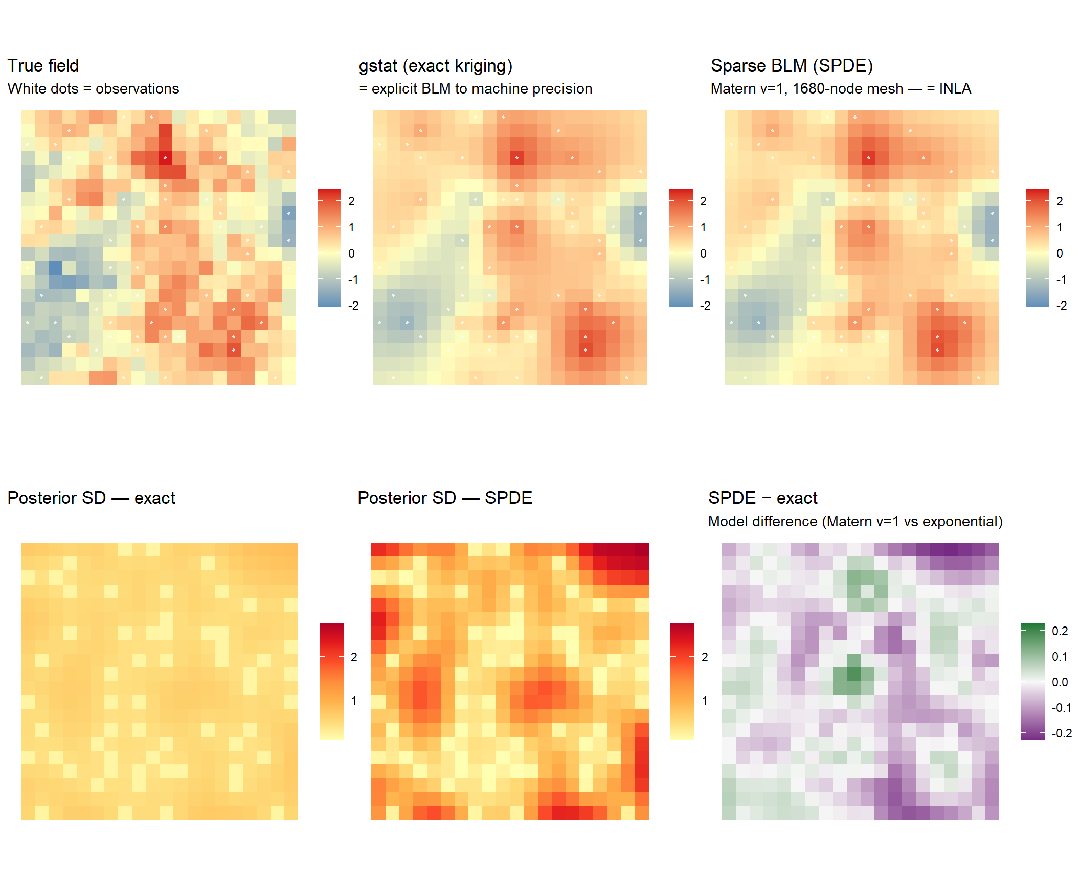
What the code is doing

Both parts are a direct transcription of \((A^\top \Sigma^{-1} A + Q)^{-1} A^\top \Sigma^{-1} y\). The only difference between Part 1 and Part 2 is the structure of \(Q\) — dense in Part 1, sparse in Part 2. The formula, and therefore the code, is identical. This is the content of the claim: kriging is Bayesian linear regression, not merely analogous to it.

Nuggets and measurement error in gstat

gstat by default treats the nugget as microscale spatial variation and interpolates exactly through observations — the aleatoric interpretation from the nugget section above. The Err model tells gstat to treat \(\sigma^2_\varepsilon\) as measurement error instead, enabling smoothing.

Scaling up with fastblm

The explicit code above works for moderate \(n\) and \(r\). For satellite datasets with large \(n\) and fine meshes, forming \(K\) explicitly is infeasible. The fastblm package implements the same posterior mean formula with PCG iterative solvers, Woodbury for the \(p \gg n\) case, and cross-validation for parameter estimation. The Boston albedo demo below uses fastblm with spatintegrate for areal observations — replacing \(A_{ij} = \frac{1}{|B_i|}\int_{B_i}\phi_j(s)\,ds\) with a precomputed sparse matrix from satellite footprint geometries.

References

Ambikasaran, Sivaram, Daniel Foreman-Mackey, Leslie Greengard, David W. Hogg, and Michael O’Neil. 2016. “Fast Direct Methods for Gaussian Processes.” IEEE Transactions on Pattern Analysis and Machine Intelligence 38 (2): 252–65.

Banerjee, Sudipto, Alan E. Gelfand, Andrew O. Finley, and Huiyan Sang. 2008. “Gaussian Predictive Process Models for Large Spatial Data Sets.” Journal of the Royal Statistical Society: Series B 70 (4): 825–48. https://doi.org/10.1111/j.1467-9868.2008.00663.x.

Chilès, Jean-Paul, and Nicolas Desassis. 2018. “Fifty Years of Kriging.” In Handbook of Mathematical Geosciences, edited by B. S. Daya Sagar, Qiuming Cheng, and Frits Agterberg, 589–612. Cham: Springer.

Cressie, Noel A. C. 1993. Statistics for Spatial Data. Revised. New York: Wiley.

Cressie, Noel, and Gardar Johannesson. 2008. “Fixed Rank Kriging for Very Large Spatial Data Sets.” Journal of the Royal Statistical Society: Series B 70 (1): 209–26. https://doi.org/10.1111/j.1467-9868.2007.00633.x.

Datta, Abhirup, Sudipto Banerjee, Andrew O. Finley, and Alan E. Gelfand. 2016. “Hierarchical Nearest-Neighbor Gaussian Process Models for Large Geostatistical Datasets.” Journal of the American Statistical Association 111 (514): 800–812. https://doi.org/10.1080/01621459.2015.1044091.

Diggle, Peter J., and Paulo Justiniano Ribeiro. 2007. Model-Based Geostatistics. New York: Springer.

Finley, Andrew O., Abhirup Datta, Bruce D. Cook, Douglas C. Morton, Hans E. Andersen, and Sudipto Banerjee. 2019. “Efficient Algorithms for Bayesian Nearest Neighbor Gaussian Processes.” Journal of Computational and Graphical Statistics 28 (2): 401–14. https://doi.org/10.1080/10618600.2018.1537924.

Finley, Andrew O., Huiyan Sang, Sudipto Banerjee, and Alan E. Gelfand. 2009. “Improving the Performance of Predictive Process Modeling for Large Datasets.” Computational Statistics & Data Analysis 53 (8): 2873–84. https://doi.org/10.1016/j.csda.2008.09.008.

Furrer, Reinhard, Marc G. Genton, and Douglas Nychka. 2006. “Covariance Tapering for Interpolation of Large Spatial Datasets.” Journal of Computational and Graphical Statistics 15 (3): 502–23. https://doi.org/10.1198/106186006X132178.

Gramacy, Robert B., and Daniel W. Apley. 2015. “Local Gaussian Process Approximation for Large Computer Experiments.” Journal of Computational and Graphical Statistics 24 (2): 561–78. https://doi.org/10.1080/10618600.2014.914515.

Guhaniyogi, Rajarshi, and Sudipto Banerjee. 2018. “Meta-Kriging: Scalable Bayesian Modeling and Inference for Massive Spatial Datasets.” Technometrics 60 (4): 430–44. https://doi.org/10.1080/00401706.2018.1437474.

Guinness, Joseph. 2019. “Spectral Density Estimation for Random Fields via Periodic Embeddings.” Biometrika 106 (2): 267–86. https://doi.org/10.1093/biomet/asz004.

Guinness, Joseph, and Montserrat Fuentes. 2017. “Circulant Embedding of Approximate Covariances for Inference from Gaussian Data on Large Lattices.” Journal of Computational and Graphical Statistics 26 (1): 88–97. https://doi.org/10.1080/10618600.2016.1164534.

Heaton, Matthew J., Abhirup Datta, Andrew O. Finley, Reinhard Furrer, Joseph Guinness, Rajarshi Guhaniyogi, Florian Gerber, et al. 2019. “A Case Study Competition Among Methods for Analyzing Large Spatial Data.” Journal of Agricultural, Biological and Environmental Statistics 24 (3): 398–425. https://doi.org/10.1007/s13253-018-00348-w.

Journel, André G., and Charles J. Huijbregts. 1978. Mining Geostatistics. London: Academic Press.

Katzfuss, Matthias. 2017. “A Multi-Resolution Approximation for Massive Spatial Datasets.” Journal of the American Statistical Association 112 (520): 201–14. https://doi.org/10.1080/01621459.2015.1123632.

Katzfuss, Matthias, and Joseph Guinness. 2021. “A General Framework for Vecchia Approximations of Gaussian Processes.” Statistical Science 36 (1): 124–41. https://doi.org/10.1214/19-STS755.

Kaufman, Cari G., Mark J. Schervish, and Douglas W. Nychka. 2008. “Covariance Tapering for Likelihood-Based Estimation in Large Spatial Data Sets.” Journal of the American Statistical Association 103 (484): 1545–55. https://doi.org/10.1198/016214508000000959.

Kimeldorf, George S., and Grace Wahba. 1970. “A Correspondence Between Bayesian Estimation on Stochastic Processes and Smoothing by Splines.” Annals of Mathematical Statistics 41 (2): 495–502.

Lindgren, Finn, Håvard Rue, and Johan Lindström. 2011. “An Explicit Link Between Gaussian Fields and Gaussian Markov Random Fields: The Stochastic Partial Differential Equation Approach.” Journal of the Royal Statistical Society: Series B 73 (4): 423–98. https://doi.org/10.1111/j.1467-9868.2011.00777.x.

Matheron, Georges. 1962. Traité de géostatistique Appliquée, Vol. II: Le Krigeage. Paris: Bureau de Recherches Géologiques et Minières.

———. 1963. “Principles of Geostatistics.” Economic Geology 58 (8): 1246–66.

Nychka, Douglas, Soutir Bandyopadhyay, Dorit Hammerling, Finn Lindgren, and Stephan Sain. 2015. “A Multiresolution Gaussian Process Model for the Analysis of Large Spatial Datasets.” Journal of Computational and Graphical Statistics 24 (2): 579–99. https://doi.org/10.1080/10618600.2014.914946.

O’Hagan, Anthony. 1978. “Curve Fitting and Optimal Design for Prediction.” Journal of the Royal Statistical Society: Series B 40 (1): 1–42.

Rasmussen, Carl Edward, and Christopher K. I. Williams. 2006. Gaussian Processes for Machine Learning. Cambridge, MA: MIT Press.

Stein, Michael L. 1999. Interpolation of Spatial Data: Some Theory for Kriging. New York: Springer.

Stuart, Andrew M. 2010. “Inverse Problems: A Bayesian Perspective.” Acta Numerica 19: 451–559.

Vecchia, Aldo V. 1988. “Estimation and Model Identification for Continuous Spatial Processes.” Journal of the Royal Statistical Society: Series B 50 (2): 297–312. https://doi.org/10.1111/j.2517-6161.1988.tb01729.x.

Zammit-Mangion, Andrew, and Noel Cressie. 2021. “FRK: An R Package for Spatial and Spatio-Temporal Prediction with Large Datasets.” Journal of Statistical Software 98 (4): 1–48. https://doi.org/10.18637/jss.v098.i04.